


")


")

")
")
 in Excel & Google Sheets")


In this tutorial, we’ll explore the simplicity of running totals with multiple subcategories in Google Sheets.
We’ll create an array formula to consistently update and display the cumulative sum of values in a dataset, organized into various subcategories.
This method finds widespread application in scenarios such as financial tracking and project management. It proves particularly useful when you wish to monitor the evolving total within distinct subgroups of your data.
Let’s explore how to calculate the cumulative sum of project costs within subcategories for effective project management.
Sample Data and Explanation
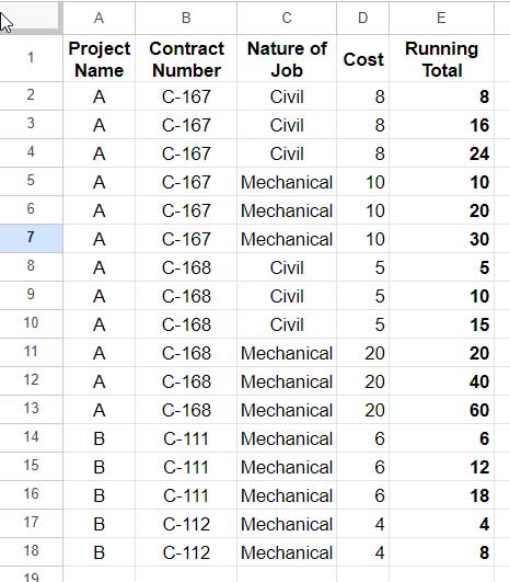
Our sample data in Google Sheets, located in the range A1:D, consists of a category column and two subcategory columns in addition to the cost column: Project Name, Contract Number, and Nature of Job.
Consider a scenario where we’ve been awarded a project and subsequently signed multiple contracts under it. For instance, the project name is ‘A,’ and the contracts under it are ‘C-167’ and ‘C-168.’
Each sub-contract is further subcategorized based on the nature of the job, resulting in subgroups like Civil, Mechanical, etc., under ‘C-167’ and ‘C-168.’
This structure extends to multiple projects. Now, we will explore how to calculate the running total by project, by project and contract numbers, and also by project, contract numbers, and type of job.
For this, you can use the SUMIFS or SUM+FILTER functions in Google Sheets. Both methods require the MAP function with a LAMBDA function to iterate over each row and return an array result.
Calculate Running Totals in Google Sheets with Subcategories
In the formula, we will include one category and two subcategories: Project Name (A2:A), Contract Number (B2:B), and Nature of Job (C2:C). These three columns will serve as criteria for calculating the running total. You can remove any of them or keep only one or two, depending on your specific needs. We will explore this later on.
The first three columns contain the categories and subcategories. The project costs are in the fourth column. So, in the fifth column, we will apply the formula that returns the running total with multiple subcategories.
We can use two Lambda formulas: One uses the SUMIFS function, and the other uses the SUM+FILTER combination. I’ll provide both and explain them.
You can obtain the sample data and formulas from the sheet provided below:
Running Total with Multiple Subcategories Using the SUMIFS Function
We will begin by crafting the non-array SUMIFS formula and subsequently convert it into an array formula for a comprehensive understanding of the logic.
Non-Array Formula
Enter the following SUMIFS formula in cell E2 and copy it down to cell E18:
=ARRAYFORMULA(SUMIFS(
   $D$2:$D,
   $A$2:$A, A2,
   $B$2:$B, B2,
   $C$2:$C, C2,
   ROW($A$2:$A), "<="&ROW(A2)
))
Syntax of the SUMIFS Function:
SUMIFS(sum_range, criteria_range1, criterion1, [criteria_range2, …], [criterion2, …])Breakdown:
sum_range: $D$2:$Dcriteria_range1: $A$2:$Acriterion1: A2criteria_range2: $B$2:$Bcriterion2: B2criteria_range3: $C$2:$Ccriterion3: C2criteria_range4: ROW($A$2:$A)criterion4: “<=”&ROW(A2)
Note: The sum_range, criteria_range4, and criterion4 are the required arguments; others are optional. However, if you remove criteria_range3, you should also remove criterion3.
The formula sums the range $D2:$D if the matching criteria are met. Absolute cell references are employed in the criteria ranges, while relative cell references are used in the criteria.
As you copy the formula down, the relative cell references within the criteria increment, while the absolute cell references defining the criteria ranges remain unchanged.
Criteria range 4 and criterion 4 work together to limit the summation, ensuring it includes only rows that are at or before the current row within the specified range. This is a crucial element in all types of cumulative sum formulas.
The ARRAYFORMULA wraps the SUMIFS formula because the ROW function is a non-array function. This ensures ROW($A$2:$A) returns a sequence of row numbers starting from row #2.
This formula calculates a running total with one category and two subcategories.
You can customize it to fit your specific needs by removing or keeping criteria columns and corresponding criteria. However, do not remove the sum range, criteria range 4, or criterion 4, as these are essential elements for the formula to function properly.
Array Formula
Copying the SUMIFS formula down increments the criteria A2, B2, C2, and "<="&ROW(A2) in each row within the range.
How can this process be automated?
To transform the aforementioned SUMIFS formula into an array formula, the MAP lambda function is employed.
Syntax:
MAP(array1, [array2, …], LAMBDA([name, …], formula_expression))MAP iterates through each element in the arrays and applies a LAMBDA function to them, generating an array of intermediate results.
Specify the criteria columns in array1, array2, array3, and name them a, b, c. Criterion 4 ("<="&ROW(A2)) doesn’t require specification as it also uses array1.
The formula_expression is the earlier SUMIFS formula, where A2 is replaced with a, B2 with b, and C2 with c.
a, b, and c serve as identifiers representing the current row within the specified range.
Here is the array formula for cell E2 to yield a running total with multiple subcategories in Google Sheets:
=MAP(
   A2:A, B2:B, C2:C, LAMBDA(a, b, c,
   ARRAYFORMULA(SUMIFS(
      $D$2:$D,
      $A$2:$A, a,
      $B$2:$B, b,
      $C$2:$C, c,
      ROW($A$2:$A), "<="&ROW(a)
   ))
))
Let’s clean this formula which involves removing dollar signs as relative and absolute references are unnecessary with the array formula. Additionally, the ARRAYFORMULA is moved to the beginning, and an extra IF statement is added to return a blank if the category is blank.
Final Formula (SUMIFS):
=ARRAYFORMULA(MAP(A2:A, B2:B, C2:C, LAMBDA(a, b, c,
      IF(a="", ,SUMIFS(
         D2:D,
         A2:A, a,
         B2:B, b,
         C2:C, c,
         ROW(A2:A), "<="&ROW(a)
      ))
)))
Running Total with Multiple Subcategories Using the SUM+FILTER Combination
To calculate a running total with multiple subcategories, we can also utilize a combination of SUM+FILTER.
If you have gone through the above SUMIFS formula and explanation, understanding this combination will be straightforward.
In both SUMIFS and FILTER, we specify the sum range.
In SUMIFS, we specify the criteria range and criterion separately. However, in FILTER, we should specify it as a condition. For example, A2:A, A in SUMIFS will become A2:A = A2 in FILTER.
Here also, we will start with the non-array formula first and then convert it into an array formula using the MAP function.
Non-Array Formula
=SUM(FILTER(
   $D$2:$D,
   $A$2:$A=A2,
   $B$2:$B=B2,
   $C$2:$C=C2,
   ROW($A$2:$A)<=ROW(A2)
))
You need to enter this formula in cell E2 and copy it down to return the running total based on one category and two subcategory columns.
Syntax of the FILTER Function:
FILTER(range, condition1, [condition2, …])Breakdown:
range: $D$2:$Dcondition1: $A$2:$A=A2condition2: $B$2:$B=B2condition3: $C$2:$C=C2condition4: ROW($A$2:$A)<=ROW(A2)
Note: The range and condition4 are the required arguments; others are optional.
Here also, you can remove the conditions (category and subcategories) to return the cumulative sum without categorization. Additionally, you can specify only the categories you want.
Array Formula
We can easily convert this non-array formula to an array formula using the MAP function as earlier. Copy the final SUMIFS formula and replace the formula_expression part with SUM(FILTER(D2:D, A2:A=a, B2:B=b, C2:C=c, ROW(A2:A)<=ROW(a))).
Final Formula (SUM+FILTER):
=ARRAYFORMULA(MAP(A2:A, B2:B, C2:C, LAMBDA(a, b, c,
      IF(a="", ,SUM(FILTER(
         D2:D,
         A2:A=a,
         B2:B=b,
         C2:C=c,
         ROW(A2:A)<=ROW(a)
      )))
)))
Conclusion
By employing the powerful formulas and techniques discussed in this article, you can gain valuable insights into your data, identify trends, and make informed decisions.
The formulas do not require a sorted dataset to return a running total by multiple subcategories. However, when you start applying this formula, consider working with a sorted range ordered by category, subcategory 1, subcategory 2, and so on.
This approach facilitates quick verification of the correctness of results at a glance.
Calculating your running total with multiple subcategories in Google Sheets empowers you to efficiently track progress within complex projects.