To return running max values in Google Sheets, we can use two types of formulas – a drag-down (copy-paste) or an array formula.
Regarding the drag-down formula, it’s simple to code using the MAX function.
In the following sequence of ten values in a column {3;5;4;6;6;8;7;9;1;1}, the running maxima are the sequence of values {3;5;5;6;6;8;8;9;9;9}.
Assume the above first set of values is in cell range B2:B11.
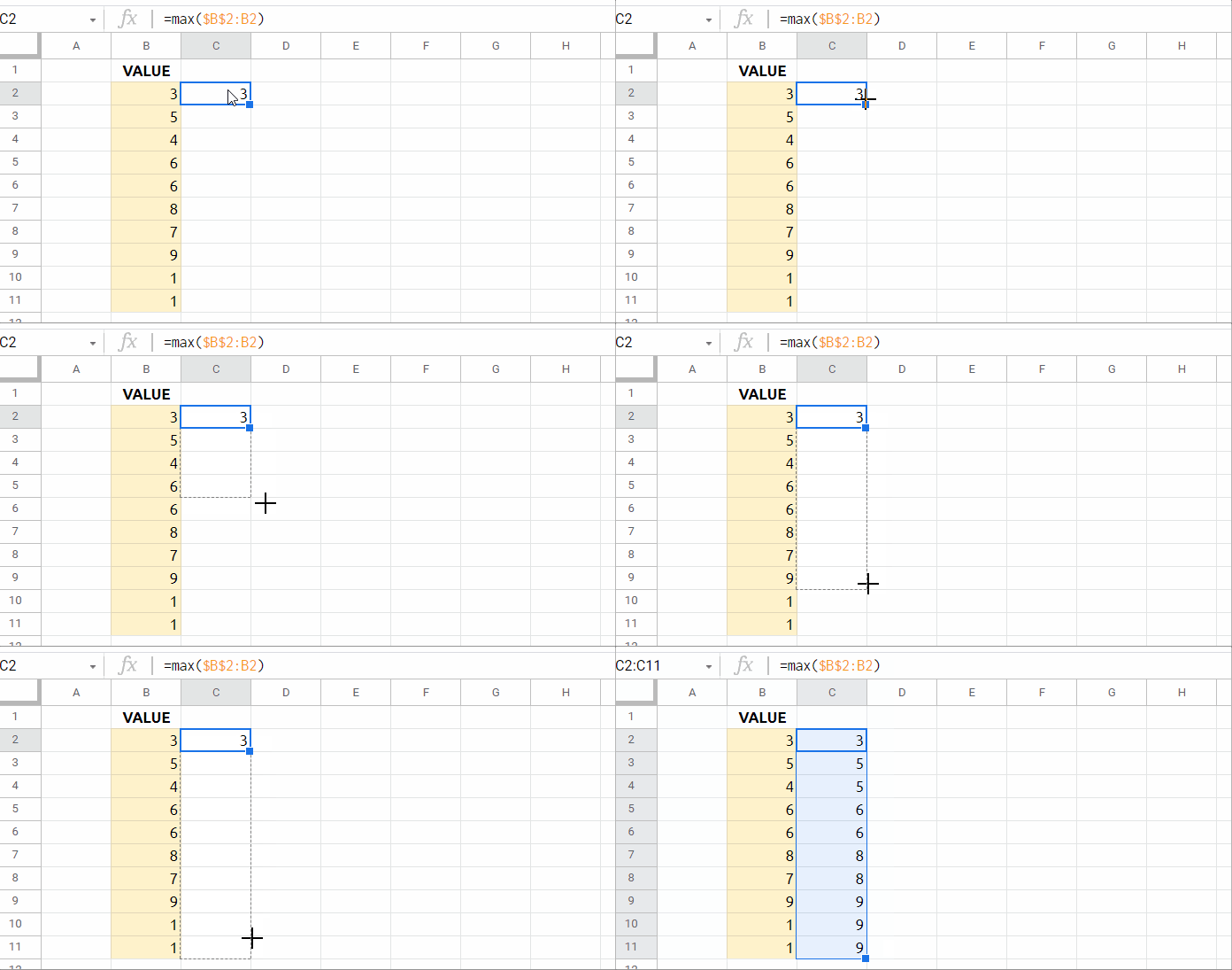
You can use the below formula in cell C2 and drag it (the fill handle in cell C2) down until C11 to get the second set, i.e., the running maxima values.
=max($B$2:B2)
As a side note, we can return High-Water Marks from the sequence of numbers in C2:C11. I’ll explain it later.
Regarding the array formula, there are different methods.
- DMAX (old)
- SCAN (new) – Recommended!
Running Max Array Formula in Google Sheets – DMAX
We can use the DMAX database function to code a running max array formula in Google Sheets. It’s somewhat complex, though.
Syntax: DMAX(database, field, criteria)
We have only a cell range (array) to use, i.e., B2:B11. So you may think that we can’t use the DMAX function.
You are correct to some extent because the said function requires a database or structured data.
To solve that, we will use some other functions to format the range to a virtual database.
The following formula may not be new to my readers.
It’s because I have used database functions for similar row-wise array results earlier.
Empty the range C2:C11 and insert the following running max array formula in cell C2.
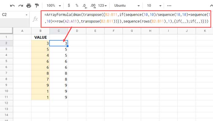
Master Running Max Array Formula:-
=ArrayFormula(dmax(transpose({B2:B11,if(sequence(10,10)/sequence(10,10)+sequence(1,10,row(A2)-1)<=row(A2:A11),transpose(B2:B11))}),sequence(rows(B2:B11),1),{if(,,);if(,,)}))
The above DMAX formula is for the values in the closed range B2:B11. Once we learn it, we will replace B11 with B (an open range).
Formula Explanation
There are three arguments in the function, and they are database, field, and criteria.
Here are them within the DMAX (only the bold part) formula above.
DATABASE
=ArrayFormula(transpose({B2:B11,if(sequence(10,10)/sequence(10,10)+sequence(1,10,row(A2)-1)<=row(A2:A11),transpose(B2:B11))}))FIELD
=ArrayFormula(sequence(rows(B2:B11),1))CRITERIA
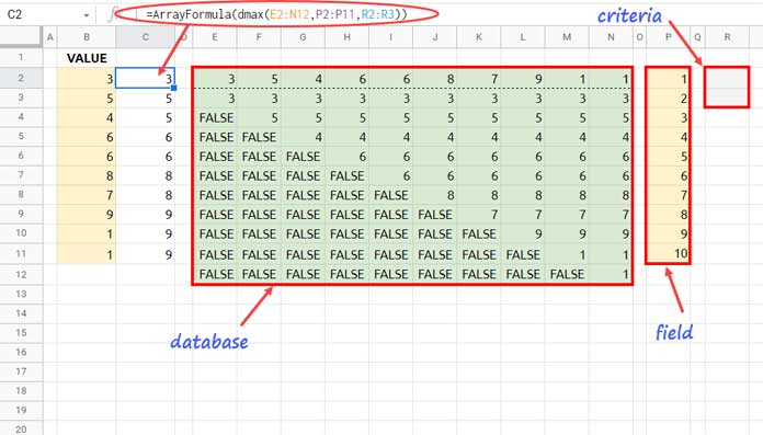
={if(,,);if(,,)}For the explanation purpose, I entered them in cells E2, P2, and R2, respectively. Please see the image below.

Note:- To make them work in standalone use, I additionally used the ArrayFormula function.
I’ve used those outputs in a new DMAX formula in cell C2 as below to return the running max of values in B2:B11.
=ArrayFormula(dmax(E2:N12,P2:P11,R2:R3))Needless to say, in our master running max array formula, we have replaced E2:N12, P2:P11, and R2:R3 with the corresponding formulas and thus avoided helper column ranges.
Arguments Explained (Field and Criteria)
I will explain the database argument later. Here are the explanations for the other two, i.e., the field and criteria.
There are ten columns in the database in E2:N12. So the field P2:P11 contains the numbers 1 to 10, which represent each column.
We have no criteria column in the database. So, as a standard in database functions, used two vertical blank cells, i.e., R2:R3, to represent it.
Related:- Two Ways to Specify Blank Cells in Google Sheets Formulas.
Now let’s go to the detail of the database, which is the core and complex part of the running max array formula in Google Sheets.
Database and Logic
I will explain the logic first to enable you to understand what’s the ‘database’ in use in E2:N12.
We can get the running max in the following way in Google Sheets.
Here are the values {3;5;4;6;6;8;7;9;1;1} in B2:B11.
To return the maximum running, we can use the formulas =max(3), =max(3,5), =max(3,5,4), =max(3,5,4,6), =max(3,5,4,6,6), =max(3,5,4,6,6,8), =max(3,5,4,6,6,8,7), =max(3,5,4,6,6,8,7,9), =max(3,5,4,6,6,8,7,9,1), =max(3,5,4,6,6,8,7,9,1,1) in cells C2, C3, C4, C5, C6, C7, C8, C9, C10, and C11, respectively.
Here the logic lies in coding the running max array formula in Google Sheets.
Let me explain it.
We will use a single formula to get the range used in the above ten max formulas in 10 columns as below.
| 3 | 3 | 3 | 3 | 3 | 3 | 3 | 3 | 3 | 3 |
| 5 | 5 | 5 | 5 | 5 | 5 | 5 | 5 | 5 | |
| 4 | 4 | 4 | 4 | 4 | 4 | 4 | 4 | ||
| 6 | 6 | 6 | 6 | 6 | 6 | 6 | |||
| 6 | 6 | 6 | 6 | 6 | 6 | ||||
| 8 | 8 | 8 | 8 | 8 | |||||
| 7 | 7 | 7 | 7 | ||||||
| 9 | 9 | 9 | |||||||
| 1 | 1 | ||||||||
| 1 |
Here is that.
=ArrayFormula(transpose({if(sequence(10,10)/sequence(10,10)+sequence(1,10,row(A2)-1)<=row(A2:A11),transpose(B2:B11))}))You may please find this formula explanation here – Get 1-12-123-1234 Patterns Using an Array Formula in Google sheets.
Now we should make it a database for DMAX.
By adding a header row, we can format the above table into a database.
So I have modified the above formula as below.
=ArrayFormula(transpose({B2:B11,if(sequence(10,10)/sequence(10,10)+sequence(1,10,row(A2)-1)<=row(A2:A11),transpose(B2:B11))}))I have just added the B2:B11 values as the field labels (even a blank row will serve the purpose).
In the above image please see the range E2:N2 for the field labels.
The above is the formula in use in cell E2 (database).
The ‘new’ DMAX in cell C2 uses the above database and returns the max of each column vertically because we have specified the fields (column numbers) vertically in P2:P11.
How to Use an Open Range in this Formula?
When we use the open range as below, the performance of our Sheet in question may be badly affected.
=ArrayFormula(if(B2:B="",,dmax(transpose({B2:B,if(sequence(rows(B2:B),rows(B2:B))/sequence(rows(B2:B),rows(B2:B))+sequence(1,rows(B2:B),row(A2)-1)<=row(A2:A),transpose(B2:B))}),sequence(rows(B2:B),1),{if(,,);if(,,)})))So, we will follow a workaround that will ensure the performance enhancements.
Here is how.
We will use a formula to find the last non-empty cell ignoring blanks in column B.
The =ArrayFormula(MATCH(2,1/(B:B<>""),1)) formula will return 11 which is the row number of the current last non-empty cell in column B.
We will use it (the bold part) to modify the running max array formula as per the below table.
| Current | To be modified to | No. of Occurrences |
B2:B11 | indirect("B2:B"&MATCH(2,1/(B:B<>""),1)) | 3 |
A2:A11 | indirect("A2:A"&MATCH(2,1/(B:B<>""),1)) | 1 |
sequence(10,10) | sequence(rows(indirect("B2:B"&MATCH(2,1/(B:B<>""),1))), | 2 |
sequence(1,10,row(A2)-1) | sequence(1,rows(indirect("B2:B"&MATCH(2,1/(B:B<>""),1))),row(A2)-1) | 1 |
I’ll make the above changes and include the formula in my sample sheet below.
Running Max Array Formula in Google Sheets – SCAN
Similar to Cummin, we can use the SCAN Lambda function for coding a running max (Cummax) array formula in Google Sheets.
Here is that formula.
=scan(B2,B2:B,lambda(a,v,if(and(a>=v,v<>""),a,v)))It has two main advantages in comparison to the previous DMAX formula.
- It’s a clean code.
- Works in a large data set.
The SCAN formula goes through the values in B2:B, from B2, row by row, replacing the values with the highest value yet, ending up with a range where the last row contains the highest value.
In the above SCAN running max array formula, a (accumulator) is equal to B2 in the first row.
Regarding v, it’s the row-by-row value to evaluate. In the first row, v will be B2, B3 in the second row, and so on.
If a>=v, the formula returns the accumulator value, else the row value. The returned max value will be the accumulator value in the next row.
High-Water Marks
The high-water marks of the present values in B2:B11 are {3;5;6;8;9}.
As far as I know, it’s the unique values of the running max values. So we are only required to wrap our array formula with UNIQUE to get it.
Syntax:- unique(running_max_formula)
Formula:-
=unique(scan(B2,B2:B,lambda(a,v,if(and(a>=v,v<>""),a,v))))That’s all. Thanks for the stay. Enjoy!


