In Google Sheets, when working with a large dataset, you might need to quickly locate specific rows—such as the row number where an item changes or where an item’s status updates. If you know the row number of a value change, you can easily navigate to it using the “Go to range” command in Google Sheets.

This tutorial explains how to find row numbers where values change and how to navigate to those rows efficiently.

Purpose

The purpose of finding the row number of a value change varies depending on the user and the dataset they are handling. For example:

• In a sales report, you might want to check the last sales quantity of an item.
• In a measurement sheet, this can help you identify the last measurement taken for a specific item.
• For status changes, you might want to find all rows where the status changed. This allows you to determine how many times each status changed and in which rows. You can then highlight or filter those rows for further analysis.

Finding the Row Numbers of Value Changes in a Column

Let’s assume you have a sales report with item names sorted in Column A. To find the row number where a specific item changes, you can use the following formula:

=ArrayFormula(XLOOKUP("orange", A1:A, ROW(A1:A), "Not Found!", 0, -1))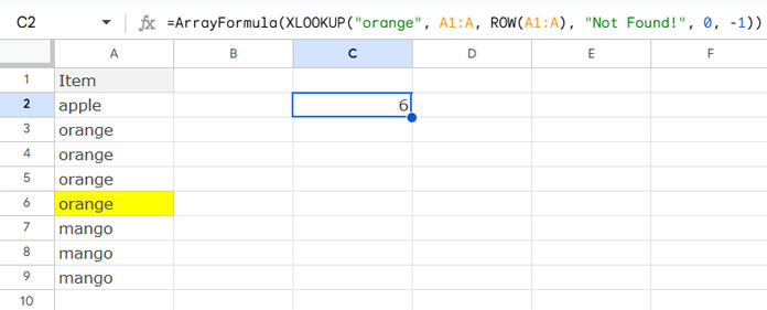

Replace “orange” with the item for which you want to find the row number of the value change.

For example, if the item “orange” last appears in row 6, the formula will return 6.

Quickly Navigating to the Value Change Row in Google Sheets

Once you have the row number of the value change, you can quickly navigate to that row by following these steps:

1. Click the Accessibility menu and select “Go to range“. Alternatively, use the keyboard shortcut:
   • Windows: Alt + /
   • Mac: Option + /
2. Enter A6 (column letter + row number of the value change).
3. Press Enter.

This will take you directly to the row where the value change occurs.

Finding the Row Numbers of Status Changes

Now, let’s find the row numbers where an order status changes. Suppose your dataset consists of two columns:

The unique statuses are Processing, Shipped, and Delivered.

To find the row numbers where the status changes for a specific order (e.g., Order ID 1001), follow these steps:

Step 1: Get Unique Statuses

Use this formula in D2 to list unique statuses:

=UNIQUE(B2:B)

Step 2: Find Row Numbers Where Status Changes

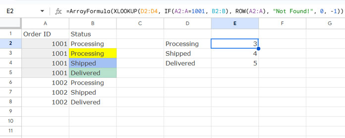
Enter this formula in E2:

=ArrayFormula(XLOOKUP(D2:D4, IF(A2:A=1001, B2:B), ROW(A2:A), "Not Found!", 0, -1))

Explanation:

• D2:D4 contains the unique statuses.
• IF(A2:A=1001, B2:B) filters the status column for Order ID 1001.
• The formula searches for each status in column B and returns the corresponding row numbers from bottom to top.

This will give you the row numbers where the status changes for Order ID 1001.

What About Column Numbers Where Values Change?

You can also use similar formulas to find the column numbers of value changes. Simply replace the ROW function with the COLUMN function. For example:

=ArrayFormula(XLOOKUP("orange", A1:Z1, COLUMN(A1:Z1), "Not Found!", 0, -1))

Additionally, if you’re using the UNIQUE function to extract unique values, ensure the syntax is correct:

=UNIQUE(range, TRUE)

Resources

Here are some related resources to help you further:

• Highlight Rows by Issue and Return Status in Google Sheets
• Filter Last Status Change Rows in Google Sheets
• Highlight Rows When Value Changes in Google Sheets
• Sum Column B Based on Changes in Column A in Google Sheets
• Highlight the Latest Value Change Rows in Google Sheets
• Reset Running Total at Every Year Change in Google Sheets (SUMIF Based)
• AT_EACH_CHANGE Named Functions for Group Totals in Sheets
• Insert a Blank Row After Each Category Change in Excel