How to Perform a Reverse HLOOKUP in Google Sheets

Reverse HLOOKUP in Google Sheets is possible. To do this, you only need to rearrange the rows ‘virtually.’ I mean there are no physical changes to the row positions—just adjustments within the HLOOKUP formula itself. How?

I’m shedding some light on this topic today. See below how to perform a reverse HLOOKUP in Google Sheets.

Table of Contents

Reverse HLOOKUP in Google Sheets – What Is It?

Normally, HLOOKUP searches across the first row for a key. In a reverse HLOOKUP, instead of the first row, we can use any other row. But remember, there is no dedicated reverse HLOOKUP function!

How is reverse HLOOKUP possible in Google Sheets?

For example, we can use HLOOKUP to search across the third row and return a value from the first row by rearranging the data within HLOOKUP. It’s very simple.

Google Sheets Reverse HLOOKUP Formula Example

See the sample data below.

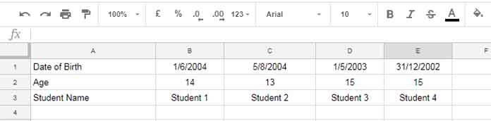
Reverse HLOOKUP example in Google Sheets

In this example, I want to find the ‘date of birth’ of “Student 2.” That means “Student 2” is the search key in HLOOKUP, but it’s located in the third row.

HLOOKUP can only search across the first row. To perform a reverse HLOOKUP in Google Sheets, first rearrange the data as shown below (this rearrangement happens within HLOOKUP):

{A3:E3; A1:E2}

Alternatively, you can use the following VSTACK formula:

VSTACK(A3:E3, A1:E2)

You should apply this as the range in your HLOOKUP formula. By doing so, Google Sheets virtually places the third row above the first row. Now, the row with the names becomes the first row, and the row containing the ‘date of birth’ becomes the second row.

In this new range, HLOOKUP becomes possible. Here’s the reverse HLOOKUP formula:

=HLOOKUP("Student 2", {A3:E3; A1:E2}, 2, FALSE)

If you used the VSTACK version for rearranging the data, the formula would be as follows:

=HLOOKUP("Student 2", VSTACK(A3:E3, A1:E2), 2, FALSE)

This formula searches across the first row for the student name “Student 2” and returns the date of birth from the second row, thanks to the rearranged data.

Note: Sometimes, formulas may return date values instead of formatted dates. If this happens, select the cells and apply Format > Number > Date to display the results correctly.

In Summary

Whenever you need to perform a reverse (or backward) HLOOKUP, simply rearrange the rows within your HLOOKUP formula.

As a side note, you can now use XLOOKUP, a modern function that allows you to specify the row to search and the result row separately, making the process much easier.

For example:

=XLOOKUP("Student 2", A3:E3, A1:E1)