You can use the RANK and FILTER functions to perform group-wise ranking in Google Sheets. This tutorial will guide you through the process.
For group-wise ranking, you typically have two columns:
- A category column may contain dates (for ranking based on dates, months, or years), or groups such as Group A, Group B, etc.
- The second column contains the numbers to be ranked.
Additionally, it’s worth noting that the data doesn’t need to be sorted in any particular order. Let’s explore how to rank groups in Google Sheets.
Rank Group Wise in Google Sheets (Rank Within Group)
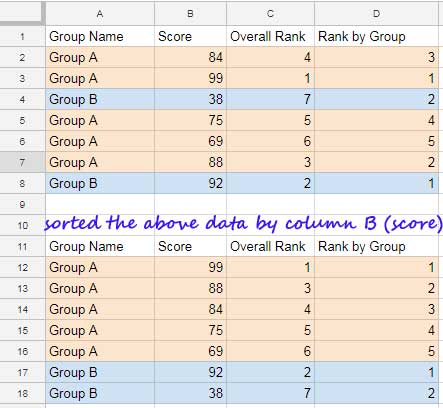
Below is a sample dataset in the range A2:B8. The first column represents the groups, while the second column contains the numbers to be ranked.
Column A consists of two groups: “Group A” and “Group B”. You can include as many groups as necessary.

The following RANK formula in cell D2, which is then copied to the range D3:D8, calculates the ranking within each group.
=RANK(B2, FILTER($B$2:B$8, $A$2:A$8=A2), 0)This adheres to the syntax: RANK(value, data, [is_ascending])
Where:
value: B2data:FILTER($B$2:B$8, $A$2:A$8=A2)
The FILTER adheres to the syntax: FILTER(range, condition), where the range is $B$2:B$8 and the condition is $A$2:A$8=A2.
is_ascending: 0
In this formula, the greatest value in each group will receive rank 1. To assign rank 1 to the lowest value, change the last parameter to 1.
=RANK(B2, FILTER($B$2:B$8, $A$2:A$8=A2), 1)To help you grasp the contrast between overall ranking and group-wise ranking, consider the sorted data presented below the original dataset, spanning from cells A12 to B18.
This sorted arrangement organizes the data based on the group in ascending order and then by the score in descending order. Examine the outcomes in column D within this sorted range.
Understanding this process should clarify how to perform ranking group-wise in Google Sheets.
RANK + Filter Combo Formula Explanation
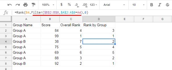
When you copy or drag the formula from cell D2 down, the formula adjusts the rank value and filter condition accordingly. For instance, consider the formula in cell D4:
=RANK(B4, FILTER($B$2:B$8, $A$2:A$8=A4), 0)
This formula filters column B based on the values in column A that match “Group B”. For row 4, the filter returns the array {38; 92}.
Thus, for row #4, you can interpret the Rank formula as follows, resulting in a rank of 2:
=RANK(38, {38; 92}, 0)Array Formula for Group-Wise Ranking
We can simplify applying the formula by using the MAP function. Clear cells D2:D8 and then insert the following array formula into cell D2:
=MAP(A2:A8, B2:B8, LAMBDA(cat, val, RANK(val, FILTER(B2:B8, A2:A8=cat), 0)))Let’s break it down step by step.
Firstly, we’ll construct a custom function using the LAMBDA function.
The syntax for the LAMBDA function is: LAMBDA(name1, name2, formula_expression)
In our case, the formula_expression will include our RANK and FILTER combination that provides the group-wise ranking. However, we’ll replace A2 and B2 (which change as we copy-paste downwards) with more meaningful names. We’ll use ‘cat’ and ‘val’ for A2 and B2, respectively.
The custom lambda function will be:
LAMBDA(cat, val, RANK(val, FILTER(B2:B8, A2:A8=cat), 0))Next, the syntax for the MAP function is as follows: MAP(array1, array2, lambda)
We’ll replace lambda with the custom lambda function we created above, and specify A2:A8 and B2:B8 in array1 and array2.
The MAP function will enable the lambda function to iterate over each value in the arrays A2:A8 and B2:B8, assigning ‘cat’ and ‘val’ to each corresponding value, respectively.
What About Dates in a Category Column?
In group-wise ranking, if the category column contains dates, you can rank based on date, month, or year.
Let’s assume A2:A8 contains dates.
For date-wise ranking, you can use the same formula as above:
=RANK(B2, FILTER($B$2:B$8, $A$2:A$8=A2), 0)
=MAP(A2:A8, B2:B8, LAMBDA(cat, val, RANK(val, FILTER(B2:B8, A2:A8=cat), 0)))
For month-wise ranking:
=RANK(B2, FILTER($B$2:B$8, EOMONTH($A$2:A$8, 0)=EOMONTH(A2, 0)), 0)
=MAP(A2:A8, B2:B8, LAMBDA(cat, val, RANK(val, FILTER(B2:B8, EOMONTH(A2:A8, 0)=EOMONTH(cat, 0)), 0)))
The EOMONTH function converts the dates in A2:A8 to end-of-the-month dates, facilitating month-wise ranking.
For year-wise ranking:
=RANK(B2, FILTER($B$2:B$8, YEAR($A$2:A$8)=YEAR(A2)), 0)
=MAP(A2:A8, B2:B8, LAMBDA(cat, val, RANK(val, FILTER(B2:B8, YEAR(A2:A8)=YEAR(cat)), 0)))
Resources
Here are some related resources.
- How to Find the Rank of a Non-Existing Number in an Existing Data Range
- Flexible Array Formula to Rank Without Duplicates in Google Sheets
- Top 10 Ranking without Duplicate Names in Google Sheets
- Compare and Highlight Up and Down in Ranking in Google Sheets
- Find the Rank of an Item in Each Column in Google Sheets
- Highlight the Top 10 Ranks in Single or Each Column in Google Sheets
- How to Rank without Ties in Google Sheets
- How to Rank Data by Alphabetical Order in Google Sheets
- How to Rank Text Uniquely in Google Sheets


