Currently, the option to print column and row headings is not available in the print menu settings in Google Sheets.
If you need to print these headings, you can follow a quick workaround. Before that, let me clarify the terms “column and row headings.”
I’ve previously explained different terms related to headings in Google Sheets. You can find more information here: Column Terminology in Google Sheets: Headings, Labels & Names.
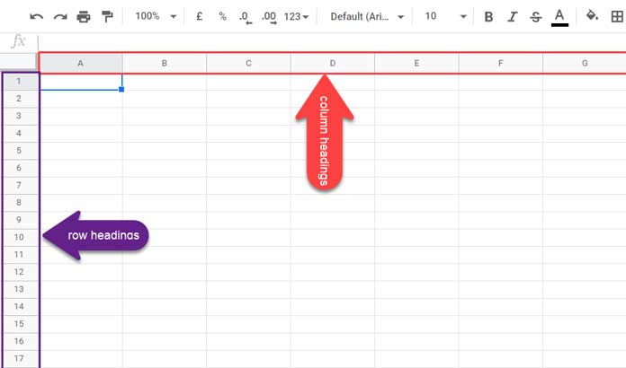
- Column headings: Letters (A, B, C, …) at the top
- Row headings: Numbers (1, 2, 3, …) on the left side
Please see the image below to understand the two headers we will discuss in this post.

In Google Sheets, the two labels marked above are outside the print area, meaning there is no way to include them within the print area as you can in Excel.
How to Print Column and Row Headings in Google Sheets: A Workaround
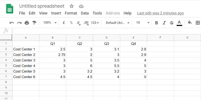
Sample Data:

Follow the steps below (in both the spreadsheet and print settings) to print the column and row headings in Google Sheets.
Spreadsheet Settings
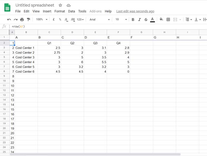
- Navigate to cell A1 and click Insert > Rows > Insert 1 row above.
- In cell A1, click Insert > Columns > Insert 1 column to the left.
- If you don’t have data, you can skip steps 1 and 2.
- Right-click on column name A and select Resize the column.
- Type 21 (to match the column width to the row height) in the given field and click OK.
- In cell A2, enter the ROW formula:
=ROW(A1). - Click and drag the fill handle (a small circle located at the bottom-right corner) down to the row where you want the row headings to print.
- In cell B1, insert the REGEXREPLACE formula:
=REGEXREPLACE(ADDRESS(1, COLUMN(A1)),"[^A-Z]", ""), and drag it across to the column where you want the column headings to appear in the print. - Click cell A2. Go to the menu View > Freeze > 1 row.

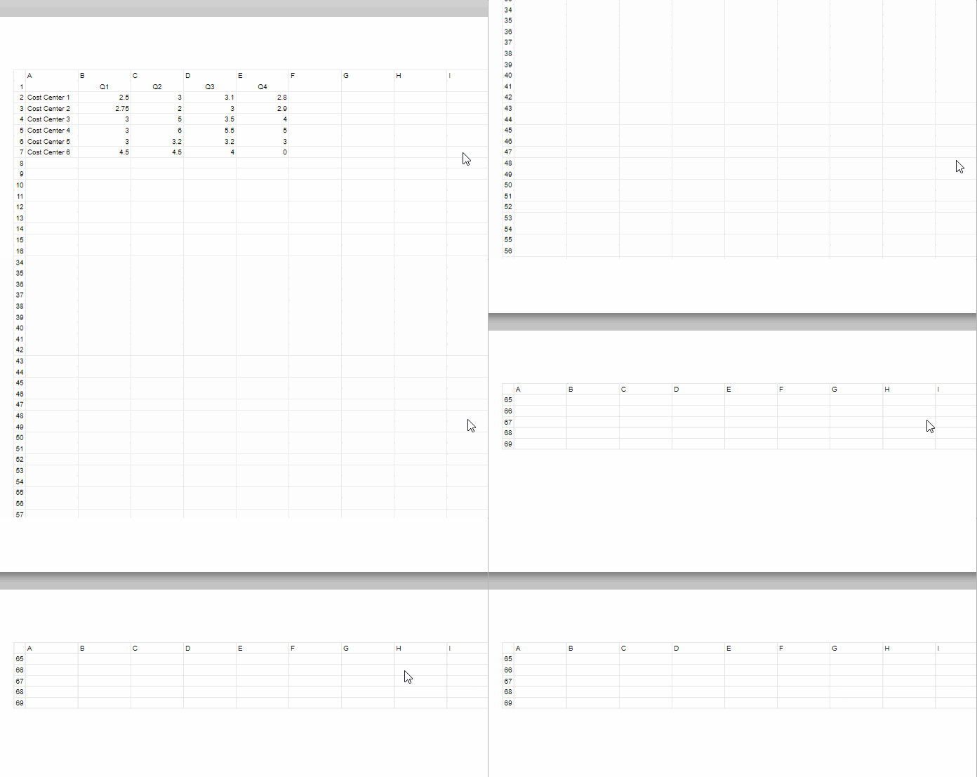
You are all set to print the column and row headings in Google Sheets.
Print Settings to Print Row and Column Headings
In Google Sheets, the print settings are accessible via the universal shortcut Ctrl + P (Windows) and Command + P (Mac), or by navigating to File > Print.
In the print settings:
- If you want, change the “Page orientation” to Portrait.
- Under the “Formatting” section of the “Print Settings,” select/enable Show Gridlines.
- Finally, under “Headers and footers,” enable Repeat frozen rows.

Resources
Here are some related Google Sheets resources:
- How to Autofill Alphabets in Google Sheets
- How to Use Roman Numbers in Google Sheets
- Clean Function in Google Sheets and Non-Printable Characters
- Freeze Pane in Google Sheets and Use It as a Header
- How to Repeat Page Titles in Google Doc Spreadsheet
- How to Add Repeat Page Titles in Google Sheets
- How to Insert Page Break in Google Sheets
- Consistent Page Numbering (X of Y) Across Multiple Sheets


