")
")


")


")

")
")
 in Excel & Google Sheets")


It’s easy to pick a random name from a lengthy list in Google Sheets. How do we keep it static, avoiding refresh with sheet changes?
Is it possible to prevent the randomly selected name from updating each time we input any value into a cell in Google Sheets?
Absolutely! This can be accomplished by leveraging LAMBDA, one of the revolutionary enhancements introduced in Google Sheets recently.
Moreover, my formula offers an additional feature.
Some users have expressed interest in avoiding repeated random names when dragging the formula downward. I have also incorporated that functionality.
Step-by-Step Instructions
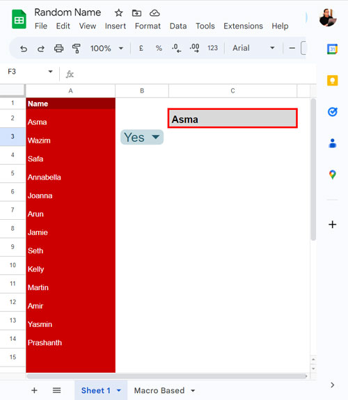
Let’s assume you have a lengthy list of student names in cells A2:A in Google Sheets. Your goal is to select a random name.
You can achieve this by using a simple formula. The formula will randomly select a name from the list in the formula cell. However, it will refresh whenever changes are made in the sheet, fetching a new name each time.
Now, let’s begin with that formula and modify it so it doesn’t refresh when changes are made to the sheet.
Basic Formula for Selecting a Random Name from a Long List
You can utilize the following formula in any cell outside the range A2:A to obtain a random name from the specified range (long list).
=INDEX(A2:A, RANDBETWEEN(1, COUNTA(A2:A)))The COUNTA function calculates the number of names in the range, while RANDBETWEEN generates a random number between 1 and the total count of names.
The INDEX function then retrieves a value by offsetting that many rows within the range.
This is the simplest method for selecting a random value from a long list in Google Sheets.
How Can I Keep the Selected Random Name Static?
I’ve highlighted the issue with the previous formula: whenever changes are made in the sheet, RANDBETWEEN refreshes, generating a new random number. Consequently, INDEX offsets by that many rows, yielding a new name.
Here are the step-by-step instructions to address this issue.
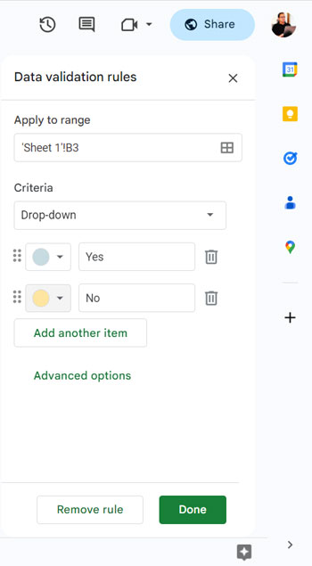
Step 1: Creating the Drop-Down:
To address this, we can introduce a drop-down box with options Yes/No to control refreshing.
- Navigate to cell B3.
- Go to the Insert menu and click Drop-down.
- Replace “Option 1” with “Yes” and “Option 2” with “No.”
- Select “Done.”
Alternatively, you can insert a Yes/No drop-down by navigating to the desired cell, typing “@”, and selecting Drop-downs > Yes/No from the context menu.
Step 2: Converting the Formula to an Unnamed Lambda Function:
Generic Formula:
=LAMBDA(x, IF($B$3="Yes", x, ""))(basic_formula)This unnamed LAMBDA function operates as follows:
If B3 equals “Yes”, return ‘x’, otherwise return blank. Here, ‘x’ represents the basic formula.
Here’s the formula to pick a random name from a list in column A and remain unchanged until you select ‘No’ in the drop-down:
=LAMBDA(x, IF($B$3="Yes", x, ""))(INDEX(A2:A, RANDBETWEEN(1, COUNTA(A2:A))))You can enhance this formula by incorporating the LET function as follows:
=LET(range, A2:A, LAMBDA(x, IF($B$3="Yes", x, ""))(INDEX(range, RANDBETWEEN(1, COUNTA(range))))In this version, we’ve assigned the name ‘range’ to A2:A.
How to Choose Multiple Unique Random Names from a Long List
The above formula is designed for selecting one random name from the list.
To pick multiple unique random names from the list, you’ll need to modify the formula as follows:
Replace A2:A with the following FILTER formula: FILTER($A$2:$A, NOT(IFERROR(XMATCH($A$2:$A, $C$1:C1))))
So the formula will be:
=LET(range, FILTER($A$2:$A, NOT(IFERROR(XMATCH($A$2:$A, $C$1:C1)))), LAMBDA(x, IF($B$3="Yes", x, ""))(INDEX(range, RANDBETWEEN(1, COUNTA(range)))))Once you’ve applied this formula to cell C2, click and drag the bottom right fill handle of cell C2 downwards to obtain more unique random names.
Important: If you encounter any issues with the formula, navigate to cell C2, copy it, delete the existing content by pressing the delete button, and then paste the copied formula.
Resources
- Google Sheets: Macro-Based Random Name Picker
- How to Randomly Select N Numbers from a Column in Google Sheets
- How to Randomly Extract a Certain Percentage of the Rows in Google Sheets
- How to Generate Odd or Even Random Numbers in Google Sheets
- Pick Random Values Based on Conditions in Google Sheets
- Interactive Random Task Assigner in Google Sheets
Thanks! your article saved me a lot of time!
Thanks a lot! Your formula was very simpler compared to the one I found from another site. However, on that site, I learned I can simply press Ctrl+R to generate another name.
Hi there,
This is a great article! I’m having an issue where I have more than one of these in the same sheet and when I change one, the other formula resets. How do I make sure that changing one Yes to No doesn’t affect the other formula?
Thanks!
Hi, Casey,
Seems you want to pick multiple random names. So instead of keeping two lists and two formulas in the same sheet, make it as one list and use another formula.
I have another tutorial. See the second link under the related post above.
Best,
Hi,
Good day!
I tried using the formula and I am sure that I have placed them in the right cells and columns. However, the picker seems to do not stop shuffling names. It runs like a loop.
How can I control the trigger? I noticed the random value changes everytime I make any change in any other cell.
How can I use the trigger only once so that the random value does not change on any other change?
It’s not possible as RANDBETWEEN is a volatile function like
now(). There may be scripts but I am not sure.The other option is trying the “Randomise range” that you can find under the Data Menu. Select the range and apply “Randomise range”
Updated: Now It’s possible to stop refreshing the generated random name.
Hey there, this worked perfectly. Just wondering, could i change the chances of a particular name coming up?
Hi, Damon,
I think you want to deliberately exclude one name appearing in the random list. In the formula replace the range A2: A (both in Index and Counta) with the filter formula as below.
filter(A2:A,A2:A<>"the name to exclude")See if this works.
Thank you for writing such an useful article. I am getting parse error whenever I try use function below in my google spreadsheet.
=if(B3=”Yes”,iferror(index(A2:A,randbetween(1,counta(A2:A))),”No Name!”),””)
It would be very helpful if you can help me in solving this problem.
Thank you in advance.
Hi Ashish,
If you copy my formula, you should retype all the double quotes in the formula. Because I’ve pasted the formulas in my post as blockquotes.
Now I’ve modified it as a code. Either retype the double quotes or copy the formula again from my page.
Hope this may solve the problem.
How do i prevent the the random name generator from using the same names more than once?
Hi,
Please see if this is working!
Randomly Select Unique N numbers