 in Google Sheets")

")

")


")


")


Currently, Google Sheets does not have a dedicated function to calculate the percentile for each group directly. However, we can achieve this using a combination of the PERCENTILE function with FILTER or IF.
Why Calculate Percentiles for Each Group?
Consider a table containing students’ marks across two different grades (or classes).
If you want to calculate the 75th percentile of all the marks, you can simply use the PERCENTILE function:
=PERCENTILE(all_marks, 0.75)However, if you need to calculate the percentile for each grade separately, the PERCENTILE function alone won’t work. Instead, we must combine it with FILTER or IF to calculate the percentile for each group in Google Sheets.
Understanding the PERCENTILE Function
Before diving into an example with marks and grades, let’s briefly explain the PERCENTILE function and how it differs from other statistical functions like AVERAGE, MIN, MAX, MEDIAN, and RANK.
- PERCENTILE returns the value below which a given percentage of data points fall.
- The 50th percentile is equivalent to the median of a dataset.
- For example, in the dataset
{5, 6}, the median is 5.5, which is also the 50th percentile.
Both PERCENTILE and MEDIAN interpolate values to determine the percentile.
How to Calculate the k-th Percentile for Each Group in Google Sheets
Understanding k-th Percentile
- The k-th percentile represents a specific value in the dataset, where k is between 0 and 1 (or 0% to 100%).
- For example, the 60th percentile can be written as
0.6or60%.
Example: Calculating the 60th Percentile for a Dataset
Sample Data:
| Student Name | Grade (Class) | Marks |
| Saul | Grade 1 | 60 |
| Allison | Grade 1 | 66 |
| Lydia | Grade 1 | 79 |
| Peter | Grade 1 | 80 |
| Sherry | Grade 1 | 79 |
| Lyle | Grade 2 | 75 |
| Adam | Grade 2 | 78 |
| Jordan | Grade 2 | 90 |
| Carlos | Grade 2 | 99 |
| Tommie | Grade 2 | 68 |
| Lola | Grade 2 | 82 |
| Cheryl | Grade 3 | 99 |
| Roger | Grade 3 | 99 |
| Angelina | Grade 3 | 97 |
| Judith | Grade 3 | 58 |
| Vicky | Grade 3 | 55 |
| Francis | Grade 3 | 90 |
To calculate the 60th percentile of all students’ marks, use:
=PERCENTILE(C2:C18, 0.6)Result: 81.20
This means 60% of students scored below 81.20 marks.
Calculating Percentile for Each Group in Google Sheets
Step 1: Get Unique Groups (Grades)
First, list unique grades using the UNIQUE function. In cell E3, enter:
=UNIQUE(B2:B)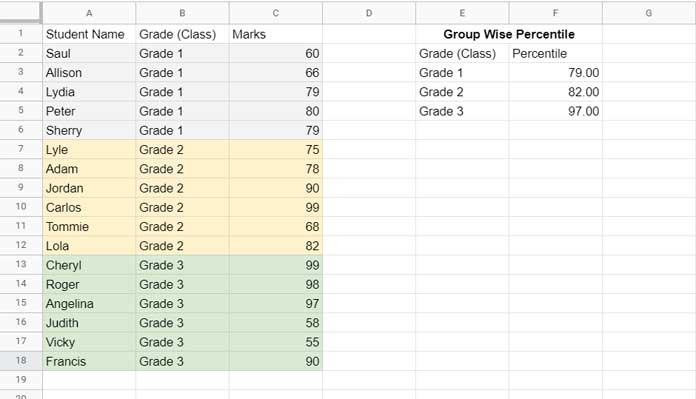
Step 2: Calculate the 60th Percentile for Each Group
Now, we calculate the percentile for each group using FILTER and PERCENTILE.
In cell F3, enter the following formula and drag it down:
=PERCENTILE(FILTER($C$2:$C, $B$2:$B=E3), 0.6)How It Works:
FILTER($C$2:$C, $B$2:$B=E3): Extracts only the marks for the current grade.PERCENTILE(..., 0.6): Calculates the 60th percentile for that group.
Alternative Method: Using PERCENTILE with IF
Instead of FILTER, you can also use IF inside an ArrayFormula:
=ArrayFormula(PERCENTILE(IF($B$2:$B=E3, $C$2:$C), 0.6))IF($B$2:$B=E3, $C$2:$C): Returns marks for the matching grade, otherwise FALSE.PERCENTILE(..., 0.6): Computes the 60th percentile.
Both formulas will return the percentile marks for Grade 1, Grade 2, and Grade 3.
Creating a Percentile Column for All Rows
If you want to calculate the percentile for each group in a new column without listing unique grades separately, modify the FILTER function criterion to use column B directly.
In cell D2, enter the following formula and drag it down to apply it to all rows:
=PERCENTILE(FILTER($C$2:$C, $B$2:$B=B2), 0.6)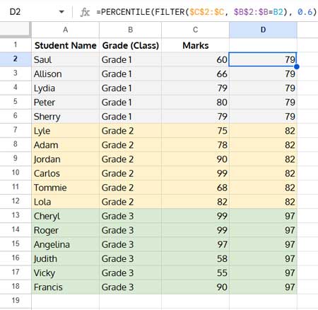
How This Works:
- The formula dynamically calculates the percentile for each student’s grade without needing a separate list of unique grades.
Note: As you can see, my sample data is sorted by category (grade), but sorting is not required for this calculation.
Frequently Asked Questions (FAQ)
1. What is the difference between PERCENTILE and PERCENTRANK in Google Sheets?
- The PERCENTILE function returns the actual value at a given percentile.
- The PERCENTRANK function returns the relative rank (as a percentage) of a value within a dataset.
- Example:
=PERCENTILE(A2:A10, 0.75)  // Returns the 75th percentile value
=PERCENTRANK(A2:A10, B2)   // Returns the rank of B2 as a percentile
2. Can I calculate percentiles without using the FILTER function?
Yes, you can use the IF function inside an ArrayFormula instead of FILTER:
=ArrayFormula(PERCENTILE(IF($B$2:$B=B2, $C$2:$C), 0.6))However, FILTER is usually more efficient and readable.
3. Can I calculate the percentile for each group dynamically?
Yes! Use the MAP function (Lambda) to get the percentile for each group on-the-fly:
=IFERROR(MAP(B2:B, LAMBDA(row, PERCENTILE(FILTER($C$2:$C, $B$2:$B=row), 0.6))))Simply enter this formula in cell D2. It automatically calculates the 60th percentile for each group and updates dynamically when new data is added.
Conclusion
By combining PERCENTILE with FILTER or IF, you can dynamically calculate the percentile for each group in Google Sheets. Whether you use a separate summary table or calculate it inline within the dataset, these methods help in statistical analysis, grading, and performance evaluation.