MINA is a statistical function in Google Sheets used to find the minimum value in a range. It differs from the MIN function. After discussing the syntax and providing a few examples, we will explore a real-life application of the MINA function in Google Sheets.

Syntax:

MINA(value1, [value2, …])

Arguments:

• value1, value2, …: These are the values or ranges to consider.

Example:

=MINA(1, 5, 4, 0)

In this example, we have used four values, and the formula will return 0 as the lowest value among them.

If these values are in A1, A2, A3, and A4, you can use:

=MINA(A1, A2, A3, A4)

or

=MINA(A1:A4)

In the latter case, we have specified the argument as a range.

How the MINA Function Differs from the MIN Function

Both the MIN and MINA functions return the smallest values from a set of values. While the former considers only numerical values in the dataset, the latter considers all values.

If the set of values contains the boolean values TRUE or FALSE, the MINA function treats them as 1 and 0, respectively. It considers text values as 0.

Therefore, the output may differ when you apply both the MIN and MINA functions in a mixed data type column.

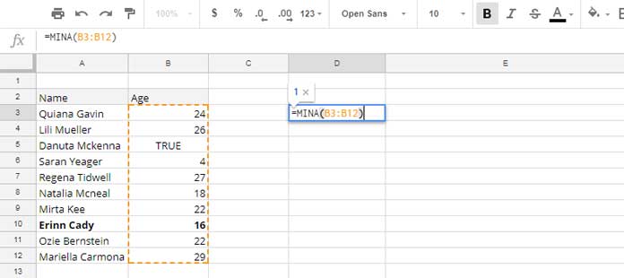
In the following example, the range B3:B12 contains numbers in all cells except B5, which contains the boolean value TRUE.

Thus, the following MINA formula in cell D3 returns 1 as the minimum value:

=MINA(B3:B13)

Practical Example of the MINA Function in Google Sheets

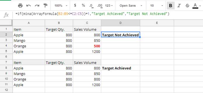
We have sales targets and actual sales in a range. Let’s test whether we meet the sales targets.

The sales targets are in B2:B5, and the actual sales are in C2:C5. The following formula will evaluate and return the status.

=IF(
   MINA(ArrayFormula(C2:C5 >= B2:B5)) = 1, 
   "Target Achieved", 
   "Target Not Achieved"
)

Formula Breakdown

The following logical part returns an array of TRUE or FALSE, where TRUE indicates that the target is met and FALSE indicates that it is not met:

=ArrayFormula(C2:C5 >= B2:B5)

We apply the MINA function to this array with:

=MINA(ArrayFormula(C2:C5 >= B2:B5))

If the output of MINA is 1, it means that all targets are met; otherwise, they are not met.

We use the IF logical test to return “Target Achieved” if the output of MINA is 1 and “Target Not Achieved” if it is 0.

Resources

• How to Exclude Zeros from MIN Function Results in Google Sheets
• Find Minimum Value and Return Value From Another Column
• How to Use MIN in Array in Google Sheets for Expanded Results
• Row-Wise MIN Using DMIN in Google Sheets
• Find Min, Max in a Matrix and Return a Value from the Same Row in Sheets
• Hyperlink Max and Min Values in Column or Row in Google Sheets
• How to Retrieve Column Header of Min Value in Google Sheets
• Get Min Date Ignoring Blanks in Each Row in Google Sheets
• Max and Min Strings Based on Alphabetic Order in Google Sheets
• Filter Min or Max Value in Each Group in Google Sheets
• Find the Running Minimum Value in Google Sheets