In this tutorial, I’ll explain how to limit the expansion of an array formula to a specific row, such as a row labeled “Total” in Google Sheets.
Normally, you can use either a closed range like A2:A100 or an open range like A2:A in Google Sheets. However, in some cases, you may want to stop the formula from expanding past a certain row or value, such as a “Total” row at the bottom of a dataset. I’ll show you how to achieve this dynamically.
Example 1: Limit Formula Expansion to the “Total” Row
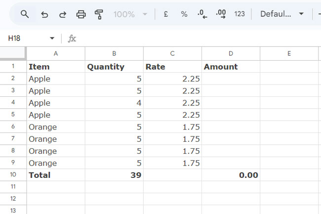
Let’s consider an example where you have a list of items in column A, their quantities in column B, and their rates in column C. The data range is A1:C9, with “Total” as a label in column A (e.g., A10).

In cell D2, I want to calculate the total amount for each item by multiplying the values in column B by the corresponding values in column C. The straightforward formula would be:
=ArrayFormula(B2:B * C2:C)However, this formula has some limitations:
It extends indefinitely down the column, preventing you from entering any values in column D.
One partial solution is to use a closed range, where you limit the expansion to the 9th row like this:
=ArrayFormula(B2:B9 * C2:C9)This way, you can place the formula =SUM(D2:D9) in cell D10 to calculate the total.
But for a more dynamic solution, you can limit the formula expansion by matching a specific value in a column (e.g., the “Total” row). This ensures the formula adjusts automatically as rows are added, without needing to manually update the ranges.
The Solution: Limit Formula Expansion Based on the “Total” Row
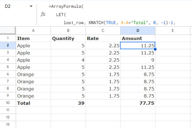
To fix this, we can limit the array formula to expand only up to the row with “Total” in column A. Here’s the solution:
=ArrayFormula(
   LET(
      last_row, XMATCH(TRUE, A:A="Total", 0, -1)-1,
      INDIRECT("B2:B"&last_row)*INDIRECT("C2:C"&last_row)
   )
)
When using this formula, replace A:A with the column that contains the specific value you want to match, thereby limiting the expansion at that value.
In our original formula, the operation is B2:B * C2:C. We modify this by replacing B2:B with INDIRECT("B2:B"&last_row) and C2:C with INDIRECT("C2:C"&last_row).
As a result, the multiplication operation B2:B * C2:C transforms into INDIRECT("B2:B"&last_row) * INDIRECT("C2:C"&last_row).
This adjustment ensures that your calculations include only the relevant rows, stopping just before the “Total” label.
Explanation:
- XMATCH: This function locates the position of the row containing “Total” in column A. The
TRUEcondition finds the match in the rangeA:A="Total"from bottom to top, and the-1outside of the XMATCH subtracts one row to ensure the formula stops before the “Total” row. - LET: This function stores the value of last_row (the row just above “Total”) and simplifies the rest of the formula. By referencing the range B2:B and C2:C dynamically up to last_row, you ensure that the formula stops expanding at the correct point.
- INDIRECT: This is used to dynamically build the range for columns B and C based on the last_row value.
Now, whenever you add rows above the “Total” row, the formula will automatically adjust to the new range.
Example 2: Expanding the Formula and Automatically Adding a Total Row
In the previous example, you would need to manually add the total calculation below the formula. Instead, we can include the total calculation directly within the formula using VSTACK to add the sum of the calculated values below the item rows.
Here’s how you can modify the formula to add the total row dynamically:
=ArrayFormula(
   LET(
      last_row, XMATCH(TRUE, A:A="Total", 0, -1)-1,
      exp, INDIRECT("B2:B"&last_row)*INDIRECT("C2:C"&last_row),
      VSTACK(exp, SUM(exp))
   )
)
Explanation:
XMATCH(TRUE, A:A="Total", 0, -1) - 1: This expression returns the last row above the “Total” row, and the defined name islast_row.INDIRECT("B2:B"&last_row) * INDIRECT("C2:C"&last_row): This is the dynamic array formula that limits the expansion of the calculation to the rows above the “Total” row, namedexp.VSTACK(exp, SUM(exp)): This function vertically stacks the calculated values (exp) along with the sum of those values (usingSUM(exp)), creating a new row with the total.
As a result, the formula will expand down to the “Total” row, and the final row will contain the sum of all item amounts. You won’t need to manually insert a total row or adjust the range every time the data changes.
Key Takeaways:
- XMATCH allows you to dynamically find a row based on a value (e.g., “Total”).
- LET simplifies complex formulas by defining and reusing variables.
- INDIRECT helps create dynamic ranges that adjust based on the dataset size.
- VSTACK is useful for adding totals or other calculations directly into the output of an array formula.
By using this method, you can make your formulas more flexible and adaptive, allowing you to limit the range and automatically account for changes in your data.
Resources
- Proper Use of MMULT in Infinite Rows in Google Sheets
- XMATCH First or Last Non-Blank Cell in Google Sheets
- Dynamic Total Row for FILTER, QUERY, or ARRAY Results in Sheets
- How to Use Dynamic Ranges in SUMIF Formula in Google Sheets
- Dynamic Ranges in Google Sheets Without Helper Cells
- How to Get Dynamic Range in Charts in Google Sheets
- Dynamic Ranges in GROWTH, TREND, and FORECAST Functions
- Average Each Row in Dynamic Range in Google Sheets
- How to Dynamically Exclude Last Empty Rows and Columns in Google Sheets
- Dynamic H&V Named Range in Google Sheets
- Adding a Dynamic Total Row to Excel FILTER Function Results
- Excel: How to Insert Subtotals Using a Dynamic Array Formula


