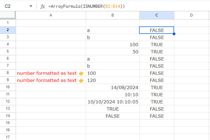
You can use the ISNUMBER function to check a cell’s content and return TRUE if it’s a number, date, or time; otherwise, it returns FALSE.

Since dates and times are represented as numeric values in Google Sheets, the ISNUMBER function will identify them as numbers. If you want to exclude dates and times, you can combine ISNUMBER with the ISDATE function. I’ll explain this combination later in the tutorial.

The ISNUMBER function is often used with logical operations, such as:

=AND(ISNUMBER(B2), B2>1)

This formula tests whether the value in cell B2 is a number and greater than 1. If you omit ISNUMBER, the formula might return TRUE even if the cell contains text. This happens because Google Sheets automatically converts text to a number when performing mathematical operations, if possible.

Syntax:

ISNUMBER(value)

• value – The cell or cell range containing the value to be verified as a number.

Formula Examples

The following formula examples will help you understand how to use the ISNUMBER function in Google Sheets.

=ISNUMBER(B2)

This formula tests the value in cell B2 and returns TRUE if it’s a number.

=ArrayFormula(ISNUMBER(B2:B14))

This formula tests the values in the cell range B2:B14 and returns an array of TRUE or FALSE values. Ensure that the cells below the formula’s range are clear to allow the array results to display correctly.

Additional Tips

By now, you may understand one of the limitations of ISNUMBER: it returns TRUE even if a cell’s content is a date, time, or datetime.

As mentioned earlier, you can use the ISDATE function in combination with ISNUMBER to address this issue.

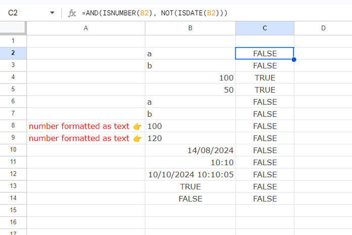
If the values are in B2:B14 and you want to return TRUE only for cells where the content is a number (not text, date, time, or datetime), enter the following formula in C2 and drag it down to C14:

=AND(ISNUMBER(B2), NOT(ISDATE(B2)))

This formula cannot be applied as an array formula because of the ISDATE function. If you want to apply it across a range, you should use the MAP function in combination with it, as follows:

=MAP(B2:B14, LAMBDA(content, AND(ISNUMBER(content), NOT(ISDATE(content)))))

ISNUMBER Function in Conditional Formatting

You can apply the ISNUMBER function in two ways in conditional formatting. If you want to test cells individually, such as A2, A2:A100, or A2:E10, use the formula:

=ISNUMBER(A2)

You should specify only the top-left cell of the range (e.g., A2) in the formula. However, apply this formula to the entire range you want to format, starting from A2. For example:

1. Select A2:E10.
2. Click Format > Conditional Formatting.
3. In the sidebar panel, ensure the “Apply to range” is A2:E10.
4. Under Format Rules, select Custom Formula Is.
5. Enter the formula =ISNUMBER(A2).
6. Click Done.

If you want to highlight an entire row when a cell’s content is a number, use this formula:

=ISNUMBER($A2)

This will highlight the entire row based on the selected range.

For example:

• If the “Apply to range” is A2:Z2, this will highlight A2:Z2 if the content in A2 is a number.
• If the “Apply to range” is A2:Z10, it will highlight each row where the content in A2:A10 is a number.

Other Related Highlight Rules:

• =ISNUMBER(A$2) – Highlights columns in the selected range (e.g., A2:Z100) if the cell content in the first row (A2:Z2) is a number.
• =ISNUMBER($A$2) – Highlights the entire selected range if the cell content in A2 is a number.

ISNUMBER Function in Data Validation

You can limit user entry to numbers only by applying the ISNUMBER function as a custom formula in data validation.

This follows the same principles as conditional formatting, but it restricts user input instead of evaluating and highlighting existing values.

Example:

1. Select the range A2:E10.
2. Click Data > Data Validation.
3. In the sidebar panel, click the Add Rule button.
4. Under Apply to Range, ensure the range is A2:E10 (it may show as something like Sheet1!A2:E10).
5. Under Criteria, select Custom Formula Is.
6. In the Formula field, enter:
   • =ISNUMBER(A2) – Allows only numbers in A2:E10.
   • =ISNUMBER($A2) – Allows only numbers in A2:A10 and permits any value in B2:E10 only if the corresponding cell in column A (A2:A10) contains a number.
   • =ISNUMBER(A$2) – Allows only numbers in A2:E2 and permits any value in A3:E10 only if the corresponding cell in row #2 (A2:E2) contains a number.
   • =ISNUMBER($A$2) – Permits entry in the selected range only if the cell content in A2 is a number, or only after entering a number in A2.

Resources

• How to Split a Number into Digits in Google Sheets
• Auto Serial Numbering in Google Sheets with Row Function
• How to Convert Currency Text to Number in Google Sheets
• Validate Comma Separated Numbers within a Specific Range
• How to Extract Decimal Part of a Number in Google Sheets