Converting currency-formatted text to numbers allows you to use values with currency symbols in calculations.
When you import data from web pages or other sources into Google Sheets, the column for currency values often formats as text because a currency symbol (e.g., $ or other symbols) prefixes the number.
The default currency format of your sheet is determined by the Locale settings under File > Settings.
If the imported currency format doesn’t match your sheet’s settings, those numbers will appear as text strings and won’t be useful for calculations or aggregation.
You can convert currency-formatted text to numbers in two ways: using the Find and Replace command or by applying the SUBSTITUTE or REGEXEXTRACT formulas. We’ll explore both options.
Convert Currency-Formatted Text to Numbers with Find and Replace
In the following example, the currency-formatted text is in column B, specifically B2:B6.
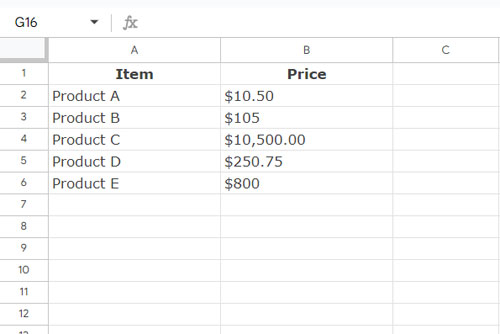
Here are the steps to convert them to numbers:
- Double-click cell B2, move the cursor to the left and select and copy the currency symbol.
- Select the range B2:B6.
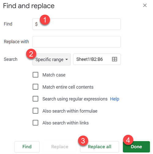
- Click Edit > Find and Replace.
- In the “Find” field, paste the copied currency symbol.
- In the “Search” field, ensure that “Specific Range” is selected from the drop-down.
- Click Replace All.
- Click Done.
This will remove the currency symbols and make the values usable in calculations.
Convert Currency-Formatted Text to Numbers with Formulas
This is an alternative strategy. We will use a helper column to apply one of the formulas below:
=ARRAYFORMULA(VALUE(SUBSTITUTE(B2:B6, "$", "")))
=ARRAYFORMULA(VALUE(REGEXEXTRACT(B2:B6, "[\d.]+")))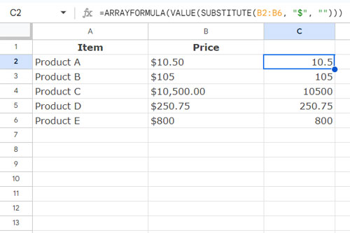
In these formulas, replace “$” with the currency symbol used in your text within the specified range.
The SUBSTITUTE in the first formula replaces “$” with an empty string, and the VALUE function converts the text-formatted numbers to numeric values.
In the second formula, the REGEXEXTRACT function extracts the numbers and the decimal point, and the VALUE function converts the extracted text to numbers.
These are the formula approaches to convert currency-formatted text to numbers in Google Sheets.
Resources
- How to Set Your Country’s Currency Format in Google Sheets
- Currency Conversion in Google Sheets Using GOOGLEFINANCE
- Lookup Dates and Return Currency Rates in an Array in Google Sheets
- Format Numbers as Currency Using Formulas in Google Sheets
- Extract Numbers Prefixed by Currency Signs from a String in Google Sheets
- Currency Formatting in Google Sheets Drop-Downs


It seems this solved the problem 🙂
=SUM(SPLIT(C1,CONCATENATE(SPLIT(C1,".0123456789"))))Hi! It looks, like what I was searching for, but I just can’t manage it 🙂
May you help me out?
I have just one text field (in C1, “1,376.77” for example) that I want to convert into a number then to shown in E1. I use this, but it doesn’t work.
=query({ArrayFormula(REGEXREPLACE(C1, "[^\d\.]+",)*1)},"Select *")Hi, Stefan,
For a single cell currency text, use my formula as below.
=REGEXREPLACE(C1, "[^\d\.]+",)*1Best,