In a string in a cell in Google Sheets, I have numbers that are with/without prefixed by currency signs. How to extract only the numbers that are prefixed by currency signs in Google Sheets?

This is a quick tutorial to share with you, I mean help to write, a Google Sheets formula for this purpose.

The formula, extracting numbers prefixed by currency signs, that I am going to write will support only any one specific currency sign.

Here I am considering the $ sign as the currency symbol. You can replace this sign with £, €, etc. depending on the sign in your string.

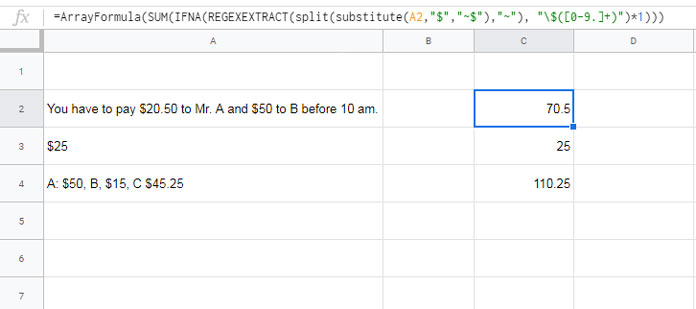
For example, the following is the string that contains Dollar signs with a few (two) numbers in cell A2.

You have to pay $20.50 to Mr. A and $50 to B before 10 am.

From this string, I just want to extract the amounts 20.50 and 50 then sum it. I don’t want to extract the last number 10 which is actually a time reference. How to do that?

With the help of (by using) REGEXEXTRACT, we can extract numbers prefixed by currency symbols from a string in Google Sheets.

Other than Regex regular expression, I am also using two more functions for this – They are SUBSTITUTE and SPLIT.

Why I am Using SUBSTITUTE and SPLIT to Extract Numbers Prefixed by Currency Signs?

You can use the regular expression \$([0-9.]+) in REGEXEXTRACT to extract the currency (Dollar) prefixed number, not numbers.

The below REGEXEXTRACT formula with the above regular expression will extract the first currency prefixed number in the given string in cell A2.

=REGEXEXTRACT(A2, "\$([0-9.]+)")

That means it would only return 20.50. What about the second, third and other occurrences if any of the currency prefixed numbers?

For that, we can use SUBSTITUTE and SPLIT with REGEXEXTRACT. We can replace the cell reference A2 in the above REGEX with a SUBSTITUTE+SPLIT combo.

The Role of SUBSTITUTE is to prefix a ~ sign before the currency prefix.

Formula:

=SUBSTITUTE(A2,"$","~$")

Output:

You have to pay ~$20.50 to Mr. A and ~$50 to B before 10 am.

The Role of SPLIT is to split the string using ~ sign as the delimiter.

Formula:

=split(substitute(A2,"$","~$"),"~")

Output:

We can use the just above combo as the cell reference in the earlier REGEXEXTRACT as it can extract currency prefixed number from a sting.

Here there are multiple (three) strings as we have split the string in the cell A2. So we must wrap the REGEXEXTRACT with ARRAYFORMULA.

=ArrayFormula(IFNA(REGEXEXTRACT(split(substitute(A2,"$","~$"),"~"), "\$([0-9.]+)")*1))

Additionally, I have used IFNA to skip unwanted #N/A errors. This formula will return the amount 20.5 and 50.

Actually any numbers extracted using REGEX will be text formatted by default. Simply multiply that number like regex output*1 to convert text to number.

Related: How to Convert Currency Text to Number in Google Sheets.

Sum Extracted Currency

If you are looking for a solution to how to extract currency prefixed numbers and sum, I can now easily provide you a formula.

Additionally, use the function SUM with the just above Google Sheets formula.

=ArrayFormula(SUM(IFNA(REGEXEXTRACT(split(substitute(A2,"$","~$"),"~"), "\$([0-9.]+)")*1)))

Further, the above formula has no issue with the currency having decimal digits.

UPDATE:

If your default currency format in Google Sheets is Dollar, then you may face one issue with Regex. I couldn’t foresee that error as my Sheets currency is set to Pound.

Here is the fix. Wrap the split output with To_Text which converts/formats numeric value to text value.

=ArrayFormula(SUM(IFNA(REGEXEXTRACT(to_text(split(substitute(A2,"$","~$"),"~")), "\$([0-9.]+)")*1)))

Additional Resources:

1. Extract All Numbers from Text and SUM It in Google Sheets.
2. How to Get Your Own Country’s Currency Format in Google Doc Spreadsheet.
3. Lookup Dates and Return Currency Rates in an Array in Google Sheets.
4. Format Numbers as Currency Using Formulas in Google Sheets.
5. How to Use the GoogleFinance Function in Google Sheets.