IMPORTRANGE to Import Visible Rows in Google Sheets

Published on

There is no argument in the IMPORTRANGE function to specify to only import visible rows from one Google Sheets file to another.

If you are new to IMPORTRANGE (I know you are not), it’s a Google Sheets function for importing a specific range of cells from one sheet to another.

With a workaround, we can import visible rows using IMPORTRANGE in Google Sheets. But it’s only possible if you have edit access to the source file to import.

Why do we require edit access?

It’s because the workaround involves an extra column (helper column) with a drag-and-drop or array formula in the source file.

Without edit access, we can’t do that in the source file.

Once you have done with those extra column settings, you can import only the visible rows using the QUERY function with IMPORTRANGE in Google Sheets.

Related Reading: How to Use Query With Importrange in Google Sheets.

In the context of this tutorial hidden rows are;

  1. Hidden rows (using the ‘Hide row’ command in the right-click shortcut menu).
  2. Collapsed row groups (using the Group rows command in the right-click shortcut menu or the View menu)
  3. Filtered out rows using the Data menu Filter command.
  4. Filtered out rows using Slicer.

Below are the step-by-step instructions to import only visible rows using IMPORTRANGE (with the help of the QUERY function) in Google Sheets.

How to Import Only Visible Rows Using IMPORTRANGE in Google Sheets?

Let’s begin with the source file settings. I am talking about adding a helper column, which I mentioned above, in the source file.

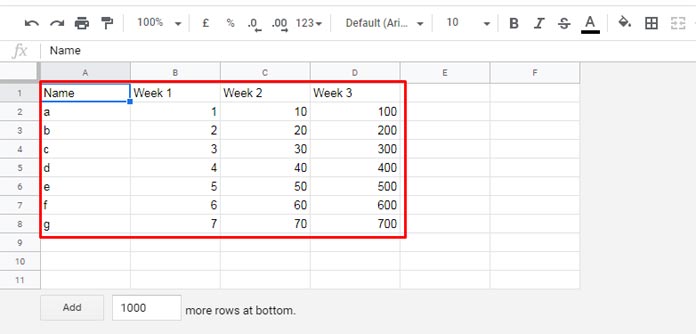
Sample Data to Import (tab name is ‘kvp1’):

Sample Data: IMPORTRANGE to Import Visible Rows

Source File Side – Helper Column Settings

  1. Make all the rows visible (already done in my sample data above). There are four methods to make a row hidden. Whatever method you have used to hide rows, unhide them using those methods.
  2. The last column that occupied data in my sheet is column D. So we can use column E as the helper column. In cell E1, insert the * formula =subtotal(103, A1) and drag it down to the table’s last row.
  3. Hide the rows you want (I am hiding rows 3, 4, and 5).

Can You Explain the Subtotal Formula in Use?

The formula I have used above is an alternative to the less popular COUNTA function, which counts values irrespective of numbers or strings.

The SUBTOTAL counta equivalent (determined by function number 103) above has one difference with COUNTA. It includes only visible rows.

For example, see the following two formulas.

=counta(A1)
=subtotal(103,A1)

Both formulas will return # 1 if cell A1 is not blank.

But when you hide row # 1, the SUBTOTAL formula will return 0, but the COUNTA won’t be affected by the hiding of the row. The output will remain 1.

You can use any non-blank column in the table (irrespective of data type.

But please ensure that the column in use doesn’t contain blank cells.

If I use A1:A8, it should not contain any blank cells.

* Update:- Instead of dragging down the E1 formula, we can now use the following auto-expanding MAP formula in E1 (first empty E1:E8).

=map(A1:A8,lambda(r,subtotal(103, r))) 

In the next step, i.e., in the destination file, we can learn to use IMPORTRANGE to import visible rows in Google Sheets. You can also learn the role of the helper column E there.

Destination File Side – QUERY IMPORTRANGE Formula to Import Visible Rows

Here are the steps to follow in the destination file to import visible rows using the IMPORTRANGE function.

  1. Copy the URL of the source file from your browser’s address bar. Paste it in cell A1 of your destination file.
  2. Enter the range (please refer to the image below) to import in cell A2. It must contain the helper column. We can later limit the columns and rows.
  3. Use the Importrange formula =importrange(A1,A2) in cell A3.

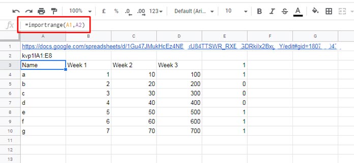
    Imported All Rows:

    Imported All Rows

    We need to specify a condition in the above IMPORTRANGE to only import the rows from the range A1:E8 if E1:E8=1.

    That we can’t do it the usual way as the function doesn’t support it.

    But we can filter the imported data for the value in destination file column E (column 5) = 1.

    As you can see in the above image, column E contains 0 in the imported data because the corresponding rows are hidden in the source file.

    That’s the point! Hidden rows have values 0 in column E because of the COUNTA equivalent SUBTOTAL(103, in the source file.

    As I mentioned at the beginning of this tutorial, there is no argument to specify conditions in IMPORTRANGE.

    The solution is using QUERY with the imported data in the destination file.

    We can combine it with the IMPORTRANGE itself.

    Related Reading: Google Sheets Query Hidden Row Handling with Virtual Helper Column.

    How Can We Use IMPORTRANGE with QUERY to Exclude Hidden Rows in the Imported Data?

    We need to modify the A3 formula as below.

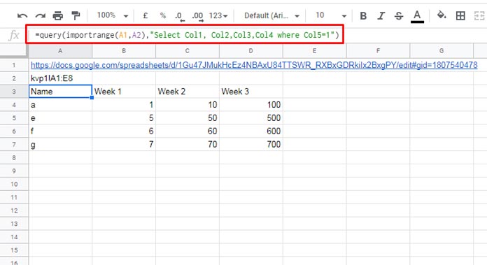
    =query(importrange(A1,A2),"Select Col1,Col2,Col3,Col4 where Col5=1")

    Imported Only Visible Rows!

    Imported Visible Rows Using IMPORTRANGE in Google Sheets

    To exclude columns, omit them in the “Select” clause, e.g., Select Col1, Col2, and Col4 to import columns A, B, and D.

    To limit the rows in the imported data use the ‘limit’ clause. You can find an example here – What is the Correct Clause Order in Google Sheets Query?

    IMPORTRANGE – Resources

    1. How to Freeze Cell in Importrange in Google Sheets [Lock Cell Reference].
    2. How to Use IMPORTRANGE Function with Conditions in Google Sheets.
    3. Dynamic Sheet Names in Importrange in Google Sheets.
    4. How to Vlookup Importrange in Google Sheets [Formula Examples].
    5. Importrange Named Ranges in Google Sheets.
    6. Dynamic Column Id in Query Importrange Using Named Ranges.
    7. Relative Cell Reference in Importrange in Sheets.
    8. Dynamic Column in Vlookup Importrange Formula in Google Sheets.
    9. Sumif Importrange in Google Sheets – Examples.
    Prashanth KV
    Prashanth KV
    Your Trusted Google Sheets and Excel Guide Prashanth KV brings a wealth of experience in Google Sheets and Excel, cultivated through years of work with multinational corporations in Mumbai and Dubai. As a recognized Google Product Expert in Docs Editors, Prashanth shares his expertise through insightful blogging since 2012. Explore his blog for practical tips and guidance on maximizing your spreadsheet skills.

    Sort Data but Keep Blank Rows in Excel and Google Sheets

    Using a dynamic array formula or the FILTER command, we can sort data and...

    Lookup Values Under Categories in Excel and Google Sheets

    We can use a combination of XLOOKUP and VLOOKUP in both Excel and Google...

    Extract Items Under a Category from the Same Column in Excel

    In Excel, you can use a combination of the XLOOKUP and DROP functions to...

    How to Create a Searchable Table in Excel Using the FILTER Function

    Finding specific records, or rows containing the required information, is straightforward in Excel using...

    More like this

    XMATCH Row by Row: Finding Values Across a Range in Google Sheets

    Using the BYROW function with XMATCH in Google Sheets allows us to match values...

    Limit Formula Expansion to a Specific Row in Google Sheets

    In this tutorial, I’ll explain how to limit the expansion of an array formula...

    3-D Referencing Structured Data Tables in Google Sheets

    When you have several tables within a single sheet—not across multiple sheets in a...

    2 COMMENTS

    LEAVE A REPLY

    Please enter your comment!
    Please enter your name here

    This site uses Akismet to reduce spam. Learn how your comment data is processed.