The PERCENTIF function in Google Sheets helps you calculate the percentage of values in a range that meet a specific condition.

Can We Use Multiple Conditions in PERCENTIF?

Yes, but it requires a workaround involving curly braces and functions like SUM and ARRAYFORMULA. We’ll explore that later in the post.

Use this function carefully to avoid misleading percentages, especially due to blank cells in the range. It’s also essential to know when to use this function appropriately.

For example, you cannot use the PERCENTIF function in Google Sheets to calculate the percentage of total marks in a test. Instead, you should use a formula like =TO_PERCENT(SUM(A1:A6)/600), where A1:A6 contains the actual scores and 600 is the total maximum marks.

Now, assume you have a list of marks and want to calculate the percentage of subjects where marks are above 90. If the student scored above 90 in 4 out of 6 subjects, you’d calculate =TO_PERCENT(4/6). The PERCENTIF function in Google Sheets can help automate this.

Previously, you may have used:

=TO_PERCENT(COUNTIF(A1:A6, ">90")/6)

Now, with the PERCENTIF function:

Syntax and Arguments

PERCENTIF(range, criterion)

• range – The set of cells to evaluate.
• criterion – The condition to test against the range.

Notes:

• The range can contain text or numbers.
• For text, enclose criteria in double quotes and optionally use wildcards like *, ?, and ~.
• For numbers, you may or may not use double quotes. Operators like >, >=, <, and <= are allowed.

Can You Use Operator Functions Like GT, LT in PERCENTIF?

Yes, though not commonly used. We’ll cover this in the examples section.

Examples of the PERCENTIF Function in Google Sheets

Numeric Range Example

Suppose you have numbers in cells B2:B10.

To calculate the percentage of values greater than 90:

=PERCENTIF(B2:B10, ">"&90)

Or simply:

=PERCENTIF(B2:B10, ">90")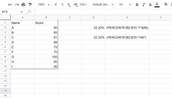

Alternative using the GT function:

=ARRAYFORMULA(PERCENTIF(GT(B2:B10, 90), TRUE))

(Not recommended for simplicity.)

You can also replicate the logic using:

=TO_PERCENT(COUNTIFS(B2:B10, ">"&90)/COUNTA(B2:B10))

Text Range Example

Suppose A2:A19 contains various text values.

To find the percentage of cells containing “Supermarket”:

=PERCENTIF(A2:A19, "Supermarket")

To include any text containing the word “Supermarket”:

=PERCENTIF(A2:A19, "*Supermarket*")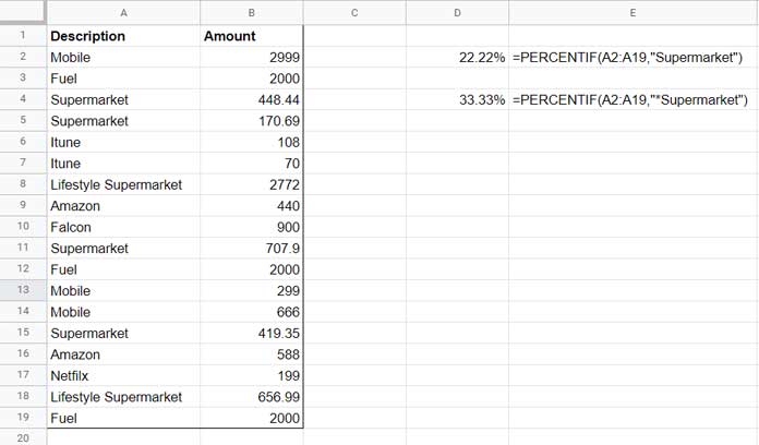

Skipping Blank Cells in PERCENTIF in Google Sheets

Avoid using open-ended ranges like B2:B or A2:A if your data includes blanks.

To filter out blanks, use either the FILTER or TOCOL function:

=PERCENTIF(FILTER(A2:A, A2:A<>""), "Supermarket")
=PERCENTIF(TOCOL(A2:A, 3), "Supermarket")

Note: This also omits any error values (e.g., #N/A), which may slightly alter results.

Using Multiple Conditions in PERCENTIF

To apply multiple conditions (e.g., “Supermarket” OR “Fuel”):

=ARRAYFORMULA(SUM(PERCENTIF(A2:A19, {"Supermarket","Fuel"})))

This method uses an array of conditions wrapped in curly braces, passed to PERCENTIF via ARRAYFORMULA, then summed.

Related Resources

• How to Calculate Reverse Percentage in Google Sheets
• Percent Distribution of Grand Total in Google Sheets Query
• Percentage Change Array Formula in Google Sheets
• Filter a Column Contains Percentage Values in Google Sheets
• Calculating the Percentage Between Dates in Google Sheets
• How to Round Percentage Values in Google Sheets
• Get Top N% Scores Per Group in Google Sheets Dynamically
• How to Calculate Percentage of Total in Google Sheets
• How to Calculate Percentage Difference in Google Sheets
• How to Limit a Percentage Value Between 0 and 100 in Google Sheets
• Calculating Percentile for Each Group in Google Sheets
• How to Use Percentage in IF Statements in Google Sheets