When you want to reverse the logical result of a condition, either on its own or within other functions, use the NOT function in Google Sheets. The NOT function inverts a logical value—returning TRUE if the input is FALSE, and FALSE if the input is TRUE.

Example:

=NOT(TRUE) // returns FALSE
=NOT(FALSE) // returns TRUE

Let’s explore this with a few examples. But first, here is the syntax of the NOT function in Google Sheets:

NOT(logical_expression)

The logical_expression can be an expression, a cell reference, or a range reference representing a logical value.

If using a range reference, remember to include the ARRAYFORMULA unless the NOT function is used within functions like SORT, SORTN, FILTER, INDEX, and SUMPRODUCT.

Basic Examples of the NOT Function in Google Sheets

If cell B2 contains “Apple”, the following logical expression will return TRUE:

=B2="Apple"

When you use this within the NOT function, the output will be FALSE:

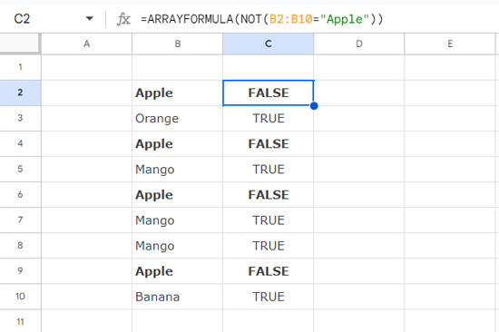
=NOT(B2:B10="Apple")

You can also use this with ARRAYFORMULA to return an array of logical values:

=ARRAYFORMULA(NOT(B2:B10="Apple"))

Real-Life Use of the NOT Function

In this example, you’ll see how to apply the NOT function in real-life scenarios in Google Sheets. We’ll start with using NOT within the FILTER function, followed by its use with XMATCH.

Example 1:

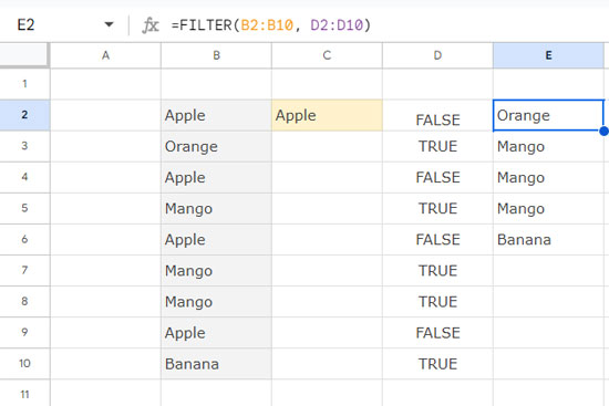
Suppose you want to extract all fruits except “Apple” in the range B2:B10. Here’s how you can do it:

Enter the condition, e.g., “Apple,” in cell C2.

In D2, enter the following formula:

=ARRAYFORMULA(NOT(B2:B10=C2))

This will return TRUE wherever the fruit in B2:B10 is not “Apple.”

In E2, enter the following FILTER formula:

=FILTER(B2:B10, D2:D10)

This filters the range B2:B10 wherever D2:D10 is TRUE, excluding “Apple.”

You can simplify this by replacing D2:D10 directly in the FILTER formula with the logic itself. When doing so, remove ARRAYFORMULA since it’s not required within the FILTER function:

=FILTER(B2:B10, NOT(B2:B10=C2))

Example 2:

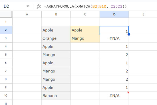
Now, let’s say you want to exclude both “Apple” (in C2) and “Mango” (in C3). To filter out both, use the XMATCH function as follows:

In D2, use this formula:

=ARRAYFORMULA(XMATCH(B2:B10, C2:C3))

This will return #N/A for any values in B2:B10 that don’t match “Apple” or “Mango” in C2:C3.

Wrap the formula with IFNA to handle errors (which can be considered as “no match” or FALSE):

=ARRAYFORMULA(IFNA(XMATCH(B2:B10, C2:C3)))

Further, wrap it with the NOT function to flip the TRUE/FALSE logic:

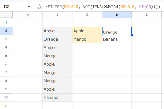
=ARRAYFORMULA(NOT(IFNA(XMATCH(B2:B10, C2:C3))))

Finally, use this within the FILTER function:

=FILTER(B2:B10, NOT(IFNA(XMATCH(B2:B10, C2:C3))))

This formula will filter out both “Apple” and “Mango” from the range B2:B10. It’s a practical approach that can be applied in many real-life scenarios, so practice with your examples!

Resources

• COUNTIFS with Not Equal to in Infinite Ranges
• AND, OR, and NOT in Conditional Formatting in Google Sheets
• How to Use Not Equal to in QUERY in Google Sheets
• How to Use AND, OR, and NOT in Google Sheets QUERY
• STARTS WITH and NOT STARTS WITH Prefix Match in QUERY
• ENDS WITH and NOT ENDS WITH Suffix Match in QUERY