Shuffling rows randomly in Google Sheets can be done using two different methods: one is formula-based, and the other is through a built-in menu option. The good news? You don’t need any plugins to do this! Let’s explore these two methods in detail and learn how to shuffle rows effectively in Google Sheets.
Before diving into the methods, let’s first highlight the key differences between them. Then, I’ll explain each approach in detail.
Formula-Based Row Shuffling in Google Sheets
If you choose the formula-based approach, it’s important to note that the data will be shuffled in a new range. We use functions like RANDARRAY with either SORT or QUERY to achieve this.
Pros:
- Non-destructive: The original data remains unchanged. The shuffled data is displayed in a separate range.
Cons:
- Volatile functions: The row order will shuffle every time Google Sheets recalculates. This may not always be desirable. However, you can limit this behavior by converting the formula into a custom LAMBDA function. This way, the data may not randomize with every edit or at specific intervals, but there’s no guarantee that it will never refresh.
Menu-Based Row Shuffling in Google Sheets
You can also shuffle rows using a Google Sheets menu option. In this case, you select the rows or data range and click a menu option to randomize the rows. I’ll show you how to do this below.
Pros:
- No volatile functions: Since no formulas are used, there are no concerns about the data reshuffling unexpectedly.
Cons:
- Changes original data: If you shuffle the rows in the same range, it will overwrite your original data, which might not be ideal in some cases.
Now, let’s walk through how to randomly shuffle rows in Google Sheets using both approaches.
How to Shuffle Rows Randomly Using Formulas in Google Sheets
Sample Data:

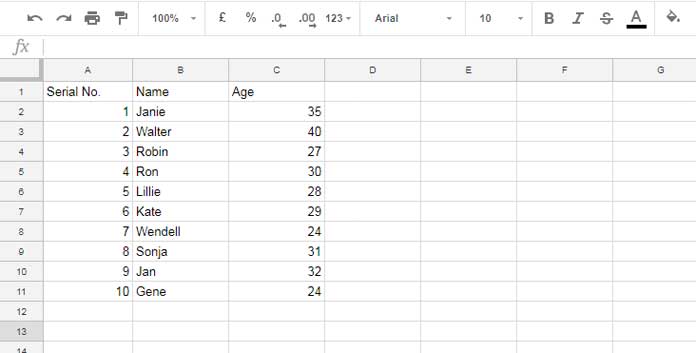
For this example, assume the data range is A1:C11, where A1:C1 is the header row. We will shuffle the rows in the range A2:C11, leaving the header row untouched.
SORT-Based Formula
To shuffle rows using the SORT function with RANDARRAY, use the following formula in cell E2:
=SORT(A2:C11, RANDARRAY(ROWS(A2:C11)), 1)- How it works:
RANDARRAY(ROWS(A2:C11)): Generates random numbers equal to the number of rows in the range.SORT(A2:C11, RANDARRAY(ROWS(A2:C11)), 1): Sorts the data inA2:C11based on the random numbers, thus shuffling the rows randomly.
Control the Auto-Shuffling Using LAMBDA
The RANDARRAY function is volatile, meaning it refreshes whenever there’s a change in the sheet or at specific intervals (which can be set under File > Settings). If you don’t want the data to reshuffle every time there’s an update, you can convert the formula into a custom unnamed LAMBDA function as follows:
=LAMBDA(randN, SORT(A2:C11, randN, 1))(RANDARRAY(ROWS(A2:C11)))This formula works similarly to the previous one but with the added flexibility of being wrapped in a LAMBDA function.
QUERY-Based Formula
Alternatively, you can use the QUERY function to shuffle rows with RANDARRAY. This approach also utilizes HSTACK to combine the random numbers with the data before sorting:
=QUERY(HSTACK(A2:C11, RANDARRAY(ROWS(A2:C11))), "SELECT Col1, Col2, Col3 ORDER BY Col4", 0)- How it works:
HSTACK(A2:C11, RANDARRAY(ROWS(A2:C11))): Horizontally stacks the original data with the random numbers.- The QUERY function then sorts the data by the random numbers (column 4), effectively shuffling the rows.
Control the Auto-Shuffling Using LAMBDA with QUERY
Just like with the SORT formula, you can also wrap the QUERY formula in a LAMBDA function to control the reshuffling:
=LAMBDA(randN, QUERY(HSTACK(A2:C11, randN), "SELECT Col1, Col2, Col3 ORDER BY Col4", 0))(RANDARRAY(ROWS(A2:C11)))Important Note
- Formula-based data: If the selected range contains any formulas, you may encounter unintended results when applying this method. Ensure the range you are shuffling only contains values (no formulas) to avoid this issue.
Menu-Based Shuffling of Rows in Google Sheet
If you prefer a simpler, non-formulaic approach, you can use Google Sheets’ built-in menu option to shuffle rows randomly.
Steps:
- Select the data range: Highlight the range
A2:C11(no need to select entire rows). - Go to the Menu: Click on
Datain the top menu. - Click on “Randomize range”: This will instantly shuffle the selected data range.
If you’re not satisfied with the initial shuffle, you can repeat this step to shuffle the rows again.
Conclusion
You now know how to shuffle rows randomly in Google Sheets using both formula-based and menu-based methods. Whether you prefer the flexibility of formulas or the simplicity of the menu option, both approaches allow you to randomize data without needing any plugins.
Each method has its own advantages and considerations, so choose the one that best fits your needs.
Resources
- Pick a Random Name from a Long List in Google Sheets
- Google Sheets: Macro Based Random Name Picker
- How to Randomly Select N Numbers from a Column in Google Sheets
- How to Randomly Extract a Certain Percentage of the Rows in Google Sheets
- How to Generate Odd or Even Random Numbers in Google Sheets
- Pick Random Values Based on Condition in Google Sheets
- Interactive Random Task Assigner in Google Sheets
- How to Generate Random Groups in Google Sheets


