Highlight Text Only in Google Sheets

Published on

We can use the ISTEXT function to highlight text entries in a range in Google Sheets. This helps identify data inconsistencies.

Highlighting text entries in a range can assist with data cleaning. Issues may arise when numbers or dates are mistakenly formatted as text, leading to invalid calculations. You can easily identify and resolve these issues by using conditional formatting to highlight text in a formula’s range.

Steps to Highlight Text Entries in a Range

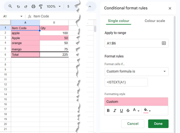
  • Select the column, row, or 2D array where the highlighting applies. For this example, we’ll select the range A1:B6.
  • Click on Format > Conditional Formatting.
  • In the sidebar panel, choose Custom Formula is under Format Rules.
  • Enter =ISTEXT(A1) (use the cell reference of the top-left cell in your selected range). For example, if you’re highlighting the range B5:B100, use =ISTEXT(B5) in the formula field.
  • Choose a fill color under the Formatting style.
  • Click Done.
Conditional formatting rule to highlight text entries in a range

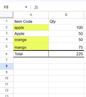
This will highlight only text entries in the selected range in Google Sheets.

Additional Tip: Highlighting Text Starting with Lowercase Letters

As part of data cleaning, you might want to highlight only text entries that start with lowercase letters.

The steps for highlighting are the same as in our previous example. The only change is in the custom formula. You can use this formula:

=AND(
   IFERROR(VALUE(A1), " ")=" ", 
   EXACT(LEFT(A1, 1), LOWER(LEFT(A1, 1)))
)
Example of highlighting text that starts with lowercase letters

Let me explain this rule:

  • IFERROR(VALUE(A1), " ") = " " – checks if the output is " ", identifying text (not numbers formatted as text).
    • IFERROR(VALUE(A1), " ") – returns " " if the cell contains text. The VALUE function produces an error when the cell contains text, and IFERROR converts that error into " ".
  • EXACT(LEFT(A1, 1), LOWER(LEFT(A1, 1)))EXACT tests if the first character in cell A1 matches its lowercase version. If TRUE, the text starts with a lowercase letter.

The AND function ensures that both conditions are met: the cell contains text (not a number formatted as text), and it starts with a lowercase letter.

This method highlights only text entries that start with a lowercase letter.

Resources

Prashanth KV
Prashanth KV
Your Trusted Google Sheets and Excel Guide Prashanth KV brings a wealth of experience in Google Sheets and Excel, cultivated through years of work with multinational corporations in Mumbai and Dubai. As a recognized Google Product Expert in Docs Editors, Prashanth shares his expertise through insightful blogging since 2012. Explore his blog for practical tips and guidance on maximizing your spreadsheet skills.

Count Consecutive Duplicates in Excel (Dynamic Array Formula)

Counting consecutive duplicates in Excel is useful for analyzing patterns, detecting repetitive sequences, and...

How to Break RANK Ties Alphabetically in Google Sheets

The RANK function in Google Sheets is commonly used to assign rankings to numerical...

Google Sheets: Highlight an Entire Column If Any Cell Has an Error

Google Sheets allows you to highlight an entire column if any cell has an...

Filter Top N per Category in Excel (Using FILTER & COUNTIFS)

You can use a combination of FILTER and COUNTIFS to filter the top N...

More like this

How to Break RANK Ties Alphabetically in Google Sheets

The RANK function in Google Sheets is commonly used to assign rankings to numerical...

Google Sheets: Highlight an Entire Column If Any Cell Has an Error

Google Sheets allows you to highlight an entire column if any cell has an...

Google Sheets: Extract Top N per Group from Query Aggregation

When working with grouped and aggregated data in Google Sheets, you might need to...

LEAVE A REPLY

Please enter your comment!
Please enter your name here

This site uses Akismet to reduce spam. Learn how your comment data is processed.