To highlight the top 10 ranks in Google Sheets, we can use the RANK or LARGE functions.

These formulas allow us to highlight up to rank 10 in a single column or, if there are values in multiple columns, in each column separately.

If there are multiple columns to highlight, we should carefully use the dollar sign ($) to apply relative and absolute references correctly in the formula.

When done correctly, there is no need to adjust the formula based on the number of columns. A single-column highlight rule will automatically adapt to the selected ranges (columns) for highlighting.

This post describes both methods (RANK and LARGE) to highlight the top 10 ranks (values) in Google Sheets.

Using the RANK Formula to Highlight Top 10 Ranks in Columns

Single Column

Let’s start with a single column. The values to highlight up to the top 10 ranks are in B2:B, as shown below.

RANK Formula for a Single Column:

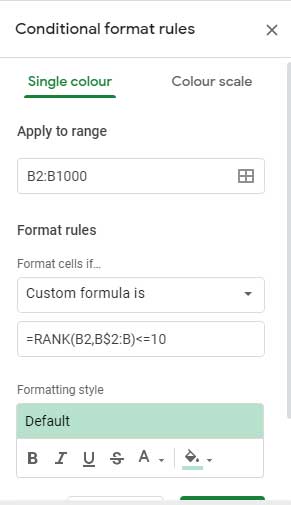
=RANK(B2, B$2:B)<=10

=RANK(B2, B$2:B$16)<=10  // If the range to highlight is B2:B16

The formula determines the rank of the value in cell B2 within the range B$2:B. Cell B2 is relative, meaning the conditional format will first determine the rank of B2, then B3, and so on within B$2:B.

Since the range B$2:B has an absolute row reference, it will remain consistent without shifting to B$3:B, B$4:B, etc.

Thus, the formula correctly highlights the top 10 ranks in the specified column. To apply this formula as a custom conditional format rule, follow these steps:

Steps:

1. Select B2:B.
2. Click Format > Conditional formatting, which will open the conditional format sidebar.
3. Ensure “Apply to range” is set to B2:B (e.g., B2:B1000 if there are 1000 rows).
4. Select “Custom formula is” under “Format rules.”
5. Enter the above RANK formula in the custom formula field.
6. Click “Done”.

If implemented correctly, the settings should resemble the screenshot below.

Each Column

To highlight the top 10 values in each column, use the same formula since absolute/relative cell references are correctly applied.

In B$2:B, only the row numbers are absolute.

Changes Required:

• If the columns to highlight are B2:B, C2:C, and D2:D, select B2:D before applying the highlighting rule or update “Apply to range” to B2:D in the sidebar panel.

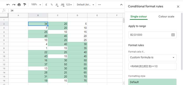
No other changes are needed.

Using the LARGE Formula to Highlight Top 10 Ranks in Columns

In Google Sheets, we can also use the LARGE function for this purpose.

=B2>=LARGE(B$2:B, 10)

This formula works for both single and multiple columns, similar to the RANK formula. The application process remains the same.

Note: Unlike RANK, the LARGE formula may not work if the number of values in the range is less than 10.

Resources

• How to Highlight Every Nth Row or Column in Google Sheets
• Highlight Earliest Events Based on Date Column in Google Sheets
• How to Highlight the Largest 3 Values in Each Row in Google Sheets
• How to Highlight an Entire Column in Google Sheets
• Highlight Every Alternate Set of N Columns in Google Sheets
• Highlight Unique Top N Values in Google Sheets
• Sales Calendar with Top 3 Highlighting in Google Sheets (Template)