Highlight the Smallest N Values in a Column in Google Sheets

Want to visually spotlight the lowest values in your data? In this tutorial, you’ll learn how to highlight the smallest N values in a column in Google Sheets using conditional formatting. Whether you’re tracking scores, expenses, or any kind of numeric data, this method helps you quickly identify the lowest performers at a glance.

Why Not Just Use the SMALL Function?

Google Sheets has a built-in SMALL function to return the Nth smallest value, but it’s not ideal for conditional formatting.

If you use it in a rule like =VALUE<=SMALL(range, n), you won’t have control over duplicates or blanks—it will highlight all values less than or equal to the Nth smallest, including repeated values.

You might think using =VALUE<=SMALL(UNIQUE(range), n) would solve the problem, but it doesn’t. This formula returns the Nth smallest unique value, which sounds helpful, but it ends up highlighting that value and all smaller values, including duplicates—not just the distinct N smallest values.

Also, if your data contains fewer than N values, the formula returns an error.

That’s why I’ve put together these custom formulas—they work reliably, even with duplicates, and give you full control over the logic for highlighting the smallest N values.

Conditional Format Rules to Highlight the Smallest N Values in a Column

Here are the rules to highlight the smallest three values in a column. Replace A$1:A$1000 with your own column range, adjust A1 to match the first cell in your range, and replace 3 with your preferred N.

Rule 1: Strict N (Exactly N Values Highlighted, Even if Duplicates Exist)

=AND(A1<>"", XMATCH(CELL("address", A1), SORTN(ADDRESS(ROW(A$1:A$1000), COLUMN(A$1:A$1000)), 3, 0, A$1:A$1000, TRUE)))

This rule highlights exactly the 3 cells with the smallest values—even if the values repeat.

How it works:

SORTN returns the addresses of the smallest 3 values. XMATCH compares each cell’s address to those returned by SORTN to decide which to highlight.

Rule 2: N + All Duplicates of the Nth Value

=RANK(A1, A$1:A$1000, TRUE)<=3

This one ranks each value in ascending order. It highlights all values that fall within the top 3, including ties with the Nth smallest value. So if the 3rd smallest value appears more than once, all its occurrences are highlighted.

How it works:

The RANK function assigns a rank to each value in the range, with the smallest value getting rank 1. The rule checks if the rank is less than or equal to 3 (or your chosen N). This means if multiple values are tied at the Nth lowest position, they all get highlighted—so it includes the N lowest values plus any ties at the Nth value.

Rule 3: N Distinct Smallest Values

=AND(XMATCH(A1, SORTN(A$1:A$1000, 3, 2, 1, TRUE)), COUNTIF(A$1:A1, A1)=1)

This highlights the 3 smallest unique values only—one instance each.

How it works:

SORTN(..., 3, 2, 1, TRUE) returns the 3 distinct smallest values. XMATCH checks if the current value exists in that list, and COUNTIF ensures only the first instance of each value gets highlighted. This rule highlights exactly 3 distinct smallest values—ignoring duplicates.

Example: Highlight the Smallest N Values in a Column in Google Sheets

Let’s say you’re tracking the number of trips to a customer over two weeks. Here’s the data (range B2:B15):

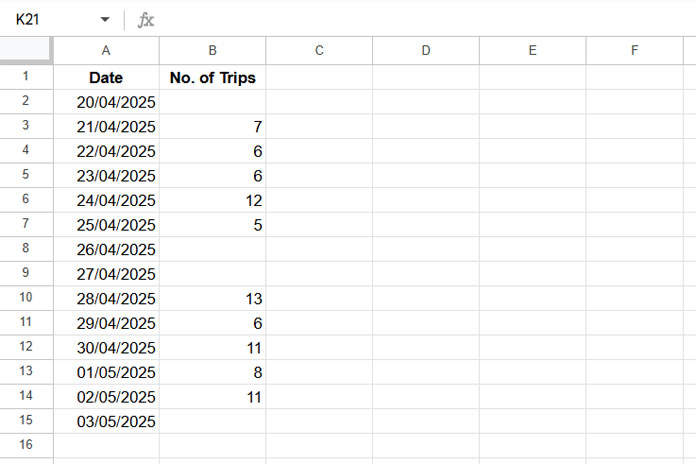
Sample data showing trip details over a two-week period in Google Sheets

Now let’s highlight the 3 lowest performing days.

Steps:

Select B2:B15.
Go to Format > Conditional Formatting.
Under Format rules, select Custom formula is.
Paste one of the formulas above, and update the cell references:
- Replace A1 with B2
- Replace A$1:A$1000 with B$2:B$1000
- Replace A$1:A1 with B$2:B2 wherever applicable.
Choose your highlight style.
Click Done.

Results:

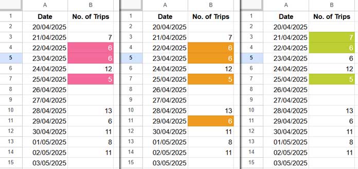
Example of highlighting the smallest N values in a column in Google Sheets

Strict 3 rule highlights: 6, 6, 5
N + ties rule highlights: 5, 6, 6, 6
Unique N rule highlights: 5, 6, 7 (if present)

How to Highlight the Smallest N Values in Each Column in a Range

The same formulas can be extended to multi-column data. Suppose you’re tracking trips for multiple crushers over two weeks (B2:D15):

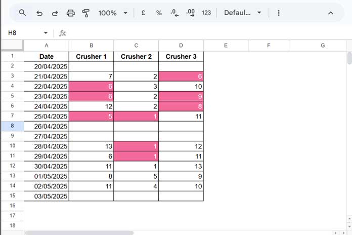
Example of highlighting the smallest N values in each column in Google Sheets

Select B2:D15 and apply your chosen formula to highlight the smallest 3 values in each column.

The only difference is the Apply to range setting. Previously, it was just B2:B15; now it should be B2:D15. The formulas remain the same.

Conclusion

Using conditional formatting with customized formulas gives you flexible ways to highlight the smallest N values in a column in Google Sheets. Whether you want to include duplicates, ignore them, or highlight every occurrence of the Nth value, there’s a formula here for your case.