


It’s very simple in Google Sheets to highlight rows when a value in any column in that row changes. With the help of conditional formatting, we can do that.
On the contrary, to sum or subtotal a column when value changes are more complex to do. I think that also you may want to know. So this tutorial is split into two parts.
The first part is on how to highlight rows when value changes in any column and the second part is on how to sum a column when value changes in another column.
Highlight Rows When Value Changes in Any Column in Google Sheets
Example:
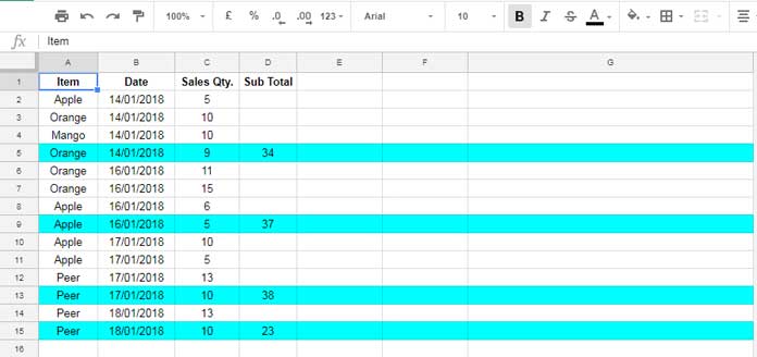
Here I’ve applied conditional formatting that would highlight the entire row when the date changes in Column B. You can find the formula to do this below.
=$B2<>$B3You can apply this formula in conditional formatting. If you are new to Google Sheets, you may want to know how to apply this formula in Conditional formatting? Below are the steps.
Steps to Follow:
Go to the menu Format > Conditional formatting…
In the Apply to range field, enter the range A2:G. Because in my data, the first row contains column labels and I’ve columns only up to column G. You can change this as per your requirement.
Under “Format cells if”, in the custom formula field, enter the above formula. Then set the colors.
This way you can highlight rows when value changes in any Column in Google Sheets.
Here instead of column B, you can set any column in the formula relevant to your data range.
In the same way, you can total a column, here column C, when value changes in Column B. As I told you, that formula is a little complex. I’ve detailed that tips in a separate tutorial – How to Total on Each Change in a Column Value.
Hope you find this Google Sheets conditional formatting tips useful. Hope to hear from you in the comments.
More Conditional Formatting Tips:
- Highlight all the Cells that contain formulas in Google Sheets.
- Indirect Function in Conditional Formatting.
- Date Related Conditional Formatting Rules in Google Sheets.
- AND, OR, or NOT in Conditional Formatting in Google Sheets.
- Multiple OR in Conditional Formatting Using Regex in Google Sheets.
Feel free to search on this page to find more awesome conditional formatting tips and tricks. Please use the search keys “Highlight” or “Conditional Formatting”.
Hi Prashanth,
I’m trying to adapt your formula to highlight changes in any column A through to and including column N but I just can’t get this correct, can you advise pls?
Hi, Debbie Grice,
I can have a try if you can share a mockup sheet similar to your working sheet.
Thank you.
This works great. Is it possible to extend this, so not just changes in 1 column e.g. column B but in a range of columns?
Thanks again.
Hi, John,
You can achieve that by combining the cells in corresponding columns.
Assume you want to highlight rows when value changes in two columns and those columns are column B and C.
Then you can go ahead with the below formula.
Best,