Do you want to search a row and column for values and highlight their intersections in Google Sheets? You can achieve this using the following formula:

=CELL("address", first_cell)=
REGEXREPLACE(CELL("address", XLOOKUP(search_key_row, first_row, first_row)), "\d" ,"")&
REGEXREPLACE(CELL("address", XLOOKUP(search_key_column, first_column, first_column)), "\D", "")

Before diving into highlighting intersections of two lookups, let’s first understand what an intersection value is.

Understanding Intersection Value in a Two-Way Lookup

Assume you have the following data in the range B2:E6:

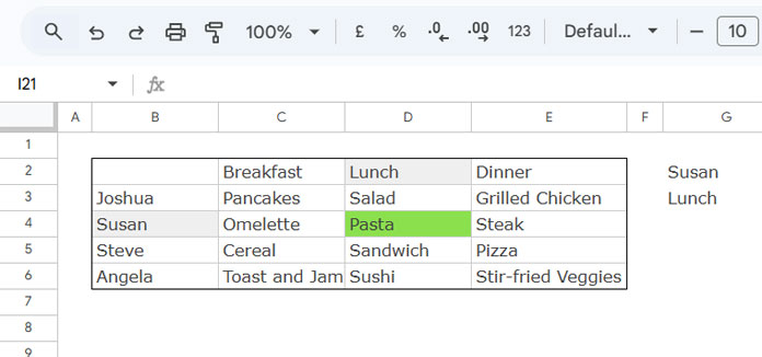
In this sample table, you can see the names of four people and their food preferences for breakfast, lunch, and dinner.

Now, assume you want to highlight the food preference of “Susan” for lunch. You’ll need to:

1. Look up “Lunch” in the first row.
2. Look up “Susan” in the first column.

This will give you the intersection value. For this example, it highlights the cell containing “Pasta”.

Example of Highlighting Intersections in Google Sheets

Follow these steps to highlight the intersection value in Google Sheets:

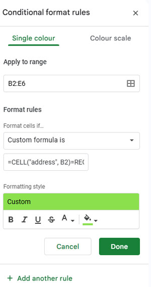
• Enter the search keys “Susan” in cell G2 and “Lunch” in cell G3
• Select the range B2:E6.
• Go to Format > Conditional Formatting.
• In the sidebar under the Single Color tab, select Custom Formula is in the “Format Rules.”
• Enter this formula in the provided field:

=CELL("address", B2)=
REGEXREPLACE(CELL("address", XLOOKUP($G$3, $B$2:$E$2, $B$2:$E$2)), "\d" ,"")&
REGEXREPLACE(CELL("address", XLOOKUP($G$2, $B$2:$B$6, $B$2:$B$6)), "\D", "")

• Choose the formatting style (e.g., fill color, text color).
• Click Done.

This will highlight the intersection value of the two lookups in Google Sheets.

How Do I Adapt This Formula to a Different Range?

To adjust this formula for another table:

• Replace B2 with the first cell in your table.
• Replace $G$3 with the search key or cell reference for the first row lookup.
• Replace $G$2 with the search key or cell reference for the first column lookup.

Modify the range references:

• Replace $B$2:$E$2 with the reference for the first row.
• Replace $B$2:$B$6 with the reference for the first column.

Maintain the relative/absolute references as in the formula to avoid errors.

The Logic Behind Highlighting Intersections in Google Sheets

The key components of this formula are the two XLOOKUP functions:

1. XLOOKUP($G$3, $B$2:$E$2, $B$2:$E$2) – Finds the match in the first row and returns the reference.
2. XLOOKUP($G$2, $B$2:$B$6, $B$2:$B$6) – Finds the match in the first column and returns the reference.

These references are passed to the CELL function to retrieve their addresses:

• CELL("address", ...) – Extracts the cell address.

We then extract the column letter and row number:

• REGEXREPLACE(..., "\d", "") – Extracts the column letter.
• REGEXREPLACE(..., "\D", "") – Extracts the row number.

Combining these gives the address of the intersection value. The formula checks if this matches the address of the current cell, highlighting it if true.

Advantage of Using XLOOKUP for Highlighting Intersections

Using XLOOKUP instead of MATCH or XMATCH avoids issues with relative positions in tables that don’t start at A1. Since XLOOKUP returns a reference or value directly, the formula works seamlessly regardless of where the table is located.

You might wonder about using VLOOKUP. However, VLOOKUP only searches vertically and cannot return a cell address when used with the CELL function.

That’s all about how to highlight intersections in Google Sheets!

Resources

• How to Perform Two-Way Lookup Using VLOOKUP in Google Sheets
• Two-Way Filter in Google Sheets: Vertical & Horizontal
• Two-way Lookup and Return Multiple Columns in Google Sheets
• Highlight VLOOKUP Results with Conditional Formatting in Sheets