A standard table usually starts with a serial number column. If your table has such a column, you can easily generate continuous numbers using the ROW function. But how do you populate group-wise serial numbers?
By “group-wise serial numbering,” I mean that the serial number should restart from 1 whenever a new group begins. In this tutorial, you’ll learn how to achieve this technique in Google Sheets.
Formula:
=SCAN(0, range, LAMBDA(a, v, IF(v="",,IF(v=OFFSET(v, IF(ROW(v)=1, 1,-1),),a+COUNTA(v), 1))))When using this formula, replace range with the cell range that contains your category data.
For example, if your category data is in the range B1:B, replace range with B1:B and apply the formula starting in the first row of an empty column (e.g., cell A1).
Example of Group-Wise Serial Numbering in Google Sheets
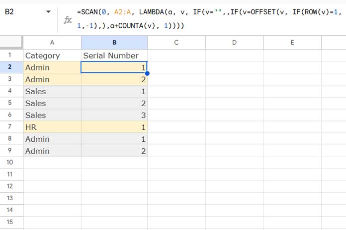
Consider the following example, where Column A contains the categories, and we want to generate the group-wise serial numbers in Column B:

In this example, the range A1:A contains the categories, and the category field label is in cell A1. The category data starts from cell A2.
The following formula in cell B2 will generate group-wise serial numbers in Column B:
=SCAN(0, A2:A, LAMBDA(a, v, IF(v="",,IF(v=OFFSET(v, IF(ROW(v)=1, 1,-1),),a+COUNTA(v), 1))))Formula Breakdown:
This formula uses the SCAN function along with a LAMBDA helper function. Here’s how it works:
SCAN(initial_value, array_or_range, lambda)initial_value: This is set to0in the formula.array_or_range: This is the rangeA2:A(where the categories are located).lambda: This function processes each element in the range.
Within the LAMBDA function:
LAMBDA(a, v, IF(v="",,IF(v=OFFSET(v, IF(ROW(v)=1, 1,-1),),a+COUNTA(v), 1)))astores the intermediate values of the SCAN operation, starting at0.vrepresents each value in the array (A2:A).
The formula does the following:
IF(v="", , ...): Checks if the current value is empty. If it’s empty, the formula returns an empty result. If it’s not empty, it proceeds to the next step.IF(v=OFFSET(v, IF(ROW(v)=1, 1, -1),), ...): Compares the current valuevwith the value in the previous row (using OFFSET). The logic here is as follows:- If
vis equal to the value in the previous row, it adds the count of occurrences ofvto the accumulatora(which is the serial number). - If the value is different from the previous row, it resets the serial number to
1.
This ensures that whenever the category changes (e.g., from “Admin” to “Sales”), the serial number restarts from1.
- If
a+COUNTA(v): Adds the count of occurrences of the current categoryvto the accumulatora(essentially counting each row in the same category).1: If the value does not match the previous row’s value, it resets the serial number to1for the new group.
How Group-Wise Serial Numbering Differs from Running Count
The key difference between this formula and a running count is how the serial number behaves when the category changes.
- Group-Wise Serial Numbering: The serial number resets to
1whenever a new group starts. If the same category (e.g., “Admin”) appears later in the column after a different group, it is treated as a new group, and the serial number starts from1again. - Running Count: A running count continues without resetting, treating all occurrences of the same category as part of the same group. When used with sorted data, it will behave like group-wise serial numbering, as the sorted order groups similar values together.
Additional Resources:
- Highlight Rows When Value Changes in Google Sheets
- Highlight the Latest Value Change Rows in Google Sheets
- Insert a Blank Row After Each Category Change in Excel
- Reverse Running Count Simplified in Google Sheets
- Fix Interchanged Names in Running Count in Google Sheets
- Running Count of Occurrences in Excel (Includes Dynamic Array)
- Case-Sensitive Running Count in Google Sheets


Hi Prashanth,
I’ve been trying to figure out how to do this for the longest time. I never considered combining match & row. This is fantastic.
Thank you so much!
Dan
Sl.No Name
1 Admin
2 Admin
1 HR
3 Admin
2 HR
Is it possible? If possible then you please sent the formula.
Hi, Nitumoni Das,
Yes! It’s possible.
Cumulative Count of All the Items in a List.
The above link will take you to the correct page in my another tutorial. There you can find a formula that would work in your above case.
I want to start 01, 02, 03 only (2 digits), if reach two digits, remove the zero.
Hi, Bajran,
You should format the numbers as below.
1. Select the range/array containing the numbers.
2. Click the menu Format > Number > More formats > Custum number format.
3. Enter
00in the blank field.