Formula to Conditionally Filter Last N Rows in Google Sheets

By using the QUERY function, you can conditionally filter the last N rows from a data range in Google Sheets. This method combines the WHERE and OFFSET clauses to achieve the result.

The WHERE clause is used to apply the required condition to filter the data. Then, with the help of the OFFSET clause, you can skip a specific number of rows from the top, effectively returning the last N rows.

Although the primary purpose of OFFSET is to skip a fixed number of rows, we can use it dynamically. That’s the trick I’ll show you in this post.

Table of Contents

Why Use Conditional Filtering on the Last N Rows?

A practical use case: Suppose you have a list of teams and their scores from the last 10 tournaments. To find the sum, average, maximum, or minimum of the last N scores of a specific team, you can apply this dynamic filtering method that returns only the relevant rows.

Example – Conditionally Filter Last N Rows in Google Sheets

GIF showing how results update when changing the N value in a formula to conditionally filter the last N rows in Google Sheets

Step 1: Apply the Condition Using `WHERE`

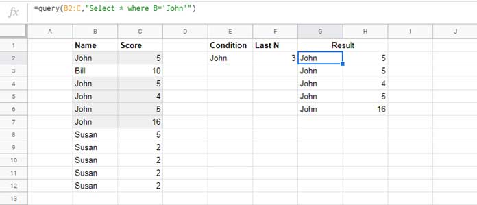
Filtering conditionally with QUERY is straightforward. For a basic example, consider filtering rows in the range B2:C where the name in column B matches a specific criterion (e.g., “John”).

Hardcoded condition:

=QUERY(B2:C, "SELECT * WHERE B = 'John'")

Dynamic condition using a cell reference (e.g., E2 contains “John”):

=QUERY(B2:C, "SELECT * WHERE B = '" & E2 & "'")

This filters rows for the specified criterion.

Example Query formula used to filter rows based on a condition in Google Sheets

Step 2: Use `OFFSET` to Filter the Last N Rows

Google Sheets’ QUERY does not have a direct clause to return the last N rows. However, by using COUNTIF and OFFSET, we can dynamically calculate how many rows to skip to get only the last N.

To find how many rows to offset:

=MAX(0, COUNTIF(B2:B, E2) - F2)

B2:B: The range to search
E2: The filter criterion (e.g., “John”)
F2: The number of rows (N) to return
MAX(0, ...): Prevents negative offset errors if N exceeds available matches

This tells us how many rows to skip (from the top) to return the last N rows for the given condition.

Now embed this logic into the full formula:

=QUERY(
  QUERY(B2:C, "SELECT * WHERE B = '" & E2 & "'"),
  "SELECT * OFFSET " & MAX(0, COUNTIF(B2:B, E2) - F2)
)

This formula performs two things:

Filters the data where column B matches E2
From the filtered results, returns the last N rows using dynamic OFFSET

Conditional SUM/AVERAGE/MAX/MIN of Last N Rows

You can extend this logic to summarize the results:

1. Conditional SUM of Last N Rows

=SUM(QUERY(
  QUERY(B2:C, "SELECT * WHERE B = '" & E2 & "'"),
  "SELECT Col2 OFFSET " & MAX(0, COUNTIF(B2:B, E2) - F2)
))

2. Conditional MAX of Last N Rows

=MAX(QUERY(
  QUERY(B2:C, "SELECT * WHERE B = '" & E2 & "'"),
  "SELECT Col2 OFFSET " & MAX(0, COUNTIF(B2:B, E2) - F2)
))

3. Conditional MIN of Last N Rows

=MIN(QUERY(
  QUERY(B2:C, "SELECT * WHERE B = '" & E2 & "'"),
  "SELECT Col2 OFFSET " & MAX(0, COUNTIF(B2:B, E2) - F2)
))

4. Conditional AVERAGE of Last N Rows

=AVERAGE(QUERY(
  QUERY(B2:C, "SELECT * WHERE B = '" & E2 & "'"),
  "SELECT Col2 OFFSET " & MAX(0, COUNTIF(B2:B, E2) - F2)
))

Error Scenarios

Be aware of two common issues:

If no matching records are found, the inner QUERY returns #N/A, which causes the full formula to error.
If F2 is blank or zero, the formula will try to return zero rows.

Conclusion

Using QUERY with WHERE and OFFSET, and combining it with COUNTIF, is a powerful way to conditionally filter the last N rows in Google Sheets. Whether you’re tracking performance, filtering reports, or performing summary calculations, this approach is flexible and dynamic.