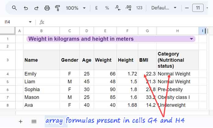
Are you health-conscious? Chances are, you are. That’s why you’ve come here to learn how to calculate BMI using a formula in Google Sheets.
The BMI formula in Google Sheets will yield the World Health Organization (WHO) recommended body mass index (BMI) levels and nutritional statuses in adults.
One significant advantage of creating a body mass indicator calculator in Google Sheets is its cloud-powered spreadsheet solution, granting you 24/7 accessibility.
The BMI formula utilizes the following categories for adults aged 20 and above:
| BMI | Category (Nutritional status) |
| Below 18.5 | Underweight |
| 18.5 to 24.9 | Normal weight |
| 25.0 to 29.9 | Pre-obesity |
| 30.0 to 34.9 | Obesity class I |
| 35.0 to 39.9 | Obesity class II |
| Above 40 | Obesity class III |
For more details, I suggest checking the relevant WHO page here.
How to Calculate BMI Using a Formula in Google Sheets
To calculate BMI in Google Sheets, you need the weight and height of the individual in question.
BMI is universally expressed in kg/m². However, in some countries, a different measuring system may be employed. If pounds and inches are used, a conversion factor of 703 must be applied (703*lb/in²).
To obtain the BMI and corresponding nutritional status (BMI category), please follow the steps below in my sample sheet (the formulas are already present in the sheet):

First, select one of the options in cell B1, which are “Weight in kilograms and height in meters” and “Weight in pounds and height in inches.”
Enter the name in cell B4, age in D4, weight, and height in cells E4 and F4 based on the value selected in the drop-down in cell B1.
The formula in cells G4 and H4 will return the BMI and nutritional status, respectively.
Both formulas are array formulas, allowing you to calculate the BMI of multiple people in one go by entering their data in the rows below.
Please continue reading to view the formulas and their explanations.
Calculating Body Mass Index: BMI Formula
The following array formula in cell G4 returns the BMI in G4:G.
=ArrayFormula(IFERROR(
      ROUND(
         IF(
            B1="Weight in kilograms and height in meters",
            E4:E/F4:F^2, 703*E4:E/F4:F^2
         ), 1
      )
))
The formula has three parts: the IF logical part, the ROUND part, and the IFERROR part. The ARRAYFORMULA function is employed as we use range references in the formula to calculate multiple BMIs in one go.
IF Logical Part:
IF(B1="Weight in kilograms and height in meters", E4:E/F4:F^2, 703*E4:E/F4:F^2)The IF function evaluates the value in cell B1, determining whether it is “Weight in kilograms and height in meters” or not. If it evaluates to TRUE, it calculates E4:E/F4:F^2, else 703*E4:E/F4:F^2.
ROUND Part:
I used the ROUND function to round the number (IF output) to 1 decimal place.
IFERROR Part:
The formula will return errors in rows where there is no height entered because the formula attempts to divide a number (weight) by 0 (height). We can assume that the row doesn’t contain a person’s data for BMI calculation. The IFERROR removes those errors.
That’s all about the BMI formula. Let’s move on to finding the nutritional status of the BMI number.
Nutritional Status: Category Identification
The following array formula in cell H4 utilizes the calculated BMI values in G4:G to determine the nutritional status.
=ArrayFormula(LET(
   bmi, G4:G,
   IF(bmi="",,
         IF(bmi<18.5, "Underweight",
            IF(bmi<=24.9, "Normal Weight",
               IF(bmi<=29.9, "Pre-obesity",
                  IF(bmi<=34.9, "Obesity class I",
                     IF(bmi<=39.9, "Obesity class II", "Obesity class III")
                  )
               )
            )
         )
   )
))
This formula is an IF logical test but nested. Instead of using G4:G, the range containing the BMI formula result, it’s named bmi and used throughout. When editing formulas, it is useful as it enables making changes in one place.
The nested IF formula is self-explanatory and employs comparison operators in the logical expressions:
IF(bmi="",– returns blank if the BMI value is emptyIF(bmi<18.5, "Underweight",– returns “Underweight” if the value is less than 18.5IF(bmi<=24.9, "Normal Weight",– returns “Normal Weight” if the value is less than or equal to 24.9IF(bmi<=29.9, "Pre-obesity",– returns “Pre-obesity” if the value is less than or equal to 29.9IF(bmi<=34.9, "Obesity class I",– returns “Obesity class I” if the value is less than or equal to 34.9IF(bmi<=39.9, "Obesity class II",– returns “Obesity class II” if the value is less than or equal to 39.9- else it returns “Obesity class III”
If desired, you can replace the category text with emojis, such as IF(bmi<=24.9, "👍"). You can copy emojis by going to Insert > Emoji.
Conclusion
I’ve explained how to calculate BMI using an array formula in Google Sheets. If you’re unfamiliar with creating the drop-down in cell B1, please refer to this guide: The Best Data Validation Examples in Google Sheets
Creating a drop-down is straightforward. Go to the Insert menu and click on drop-down. You will get a sidebar panel with options for the drop-down.
You May Also Like:


