Format Numbers as Currency Using Formulas in Google Sheets

When working with financial data in Google Sheets, it’s important to present numbers in a readable currency format. While you can use the menu option Format > Number > Currency, there’s a more dynamic and formula-driven way to format numbers as currency.

In this guide, you’ll learn how to:

Use the TO_DOLLARS and DOLLAR functions in Google Sheets
Format plain numbers as currency using formulas
Understand the difference between the two functions
Choose the right function based on your specific needs

Use Case: Calculating Total Cost in Currency Format

Assume you’re tracking purchase quantities of an item in column B, and the unit rate is $5.

Basic formula to calculate total cost:

=SUM(B2:B10) * 5

This returns a plain number, not a currency-formatted one.

To format this result as currency using a formula, wrap it with either TO_DOLLARS or DOLLAR:

=TO_DOLLARS(SUM(B2:B10) * 5)

How to Use `TO_DOLLARS` in Google Sheets

The TO_DOLLARS function converts a numeric value into your sheet’s default currency format (based on your locale).

Syntax

TO_DOLLARS(value)

Examples

=TO_DOLLARS(A1)
=ArrayFormula(TO_DOLLARS(A1:A10))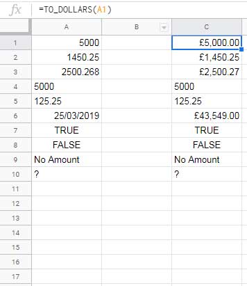

Behavior

Accepts only numeric input.
Returns output in currency format, but still a number (not text).
Returns text inputs as-is (no conversion applied).
Interprets dates as numbers—not recommended for date fields.

Pro Tip: Use TO_DOLLARS when you want the formatted result to still behave like a number (for calculations, charting, etc.).

How to Use `DOLLAR` in Google Sheets

The DOLLAR function is more flexible with input types and allows for rounding.

Syntax

DOLLAR(number, [number_of_places])

Examples

=DOLLAR(1234.567)        → "$1,234.57"
=DOLLAR(1234.567, 0)     → "$1,235"
=ArrayFormula(DOLLAR(A1:A10))

Behavior

Converts numbers and numeric text to currency format.
Returns text (not a number).
Accepts Boolean values (TRUE/FALSE) and formats them.
Throws #VALUE! error if input is pure text.

Note: Use DOLLAR when you need to display currency in text format or apply rounding.

TO_DOLLARS vs DOLLAR: Quick Comparison

Feature	`TO_DOLLARS`	`DOLLAR`
Output format	Number	Text
Accepts text input	❌ Returns as-is	✅ Converts to currency format
Works with Boolean (TRUE/FALSE)	❌ Returns as-is	✅ Formats as currency
Interprets date values	✅ Converts to currency (⚠️)	✅ Converts to currency (⚠️)
Rounding option	❌ Not available	✅ Yes, via second argument
Use in charts/calculations	✅ Recommended	❌ Not ideal (text output)

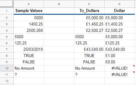
In the screenshot below, you can see how the TO_DOLLARS function (left column) and the DOLLAR function (right column) format the same input data differently. This highlights the key differences in output type, handling of text values, and formatting behavior.

Side-by-side comparison of TO_DOLLARS and DOLLAR functions in Google Sheets showing differences in currency formatting

Example: Format Total Purchase Cost as Currency

Let’s apply what we’ve learned.

Plain formula:

=SUM(B2:B10) * 5

With `TO_DOLLARS`:

=TO_DOLLARS(SUM(B2:B10) * 5)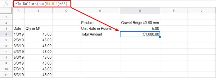

Real-life example showing how to format numbers as currency using formulas in Google Sheets

This version ensures the output remains a number in currency format, perfect for additional calculations or chart visualization.

If you need to display the value as text or round to specific decimals, use:

=DOLLAR(SUM(B2:B10) * 5, 0)

When to Use Each Function

✅ Use TO_DOLLARS when:
- You want a number output.
- You need to retain numeric behavior for formulas or charts.
- Input values are strictly numbers.
✅ Use DOLLAR when:
- You want rounded currency values.
- You’re converting numeric text to currency format.
- You’re displaying currency as plain text.