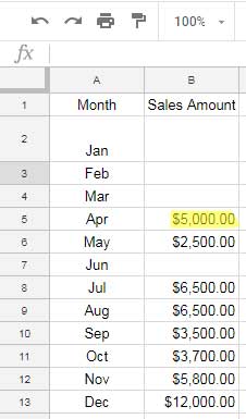
How to Return First Non-blank Value in a Row or Column in Google Sheets

In Google Sheets, you can find the first non-blank value in a row or column using either XLOOKUP or a combination of INDEX and MATCH. TOCOL and CHOOSEROWS offer another modern alternative.

This can be useful in real-life scenarios. For example, if a new employee joined your company in the middle of the year, say in June, and you want to find the first salary he received in a column containing figures from January to December, you can use this approach.

In this case, the cells from January to June will be blank, and his first salary will be in July. You can find that amount from that column without applying criteria such as employee name, month, etc.

Formulas to Return the First Non-blank Value in a Row in Google Sheets

In the following examples, we will test the formulas in row #2, specifically in the range B2:G2.

In the sample data, the values start at cell D2. So the formulas should return the value in cell D2.

Return first value in a row after skipping blank cells — Screenshot # 1

Option 1: INDEX-MATCH Combo with ISBLANK

Here is the INDEX and MATCH combo formula to return the first non-blank cell value in the row range B2:G2:

=INDEX(B2:G2, MATCH(FALSE, ISBLANK(B2:G2), 0))

Formula Breakdown

Step 1:

ISBLANK(B2:G2): The ISBLANK function returns TRUE or FALSE values corresponding to the range B2:G2. It returns TRUE for blank cells and FALSE for non-blank cells.

Syntax: ISBLANK(value)
- When using an array reference in value, you should use it as ArrayFormula(ISBLANK(value))
Where value is the range B2:G2.

Step 2:

MATCH(FALSE, ISBLANK(B2:G2), 0): The MATCH function returns the position of the first FALSE value in the step #1 result.

Syntax: MATCH(search_key, range, [search_type])
Where search_key is FALSE, range to search is ISBLANK(B2:G2), and search_type is 0, which represents an unsorted range.

Step 3:

The INDEX function offsets columns in B2:G2 according to the step #2 output and returns the value in the first FALSE (non-blank) cell.

Syntax: INDEX(reference, [row], [column])
Where reference is B2:G2 and the row / column offset is the step #2 result.

Note: The reference here is one-dimensional. If you provide a single value to offset, the function will offset rows if the reference range is vertical and columns if the reference range is horizontal.

Option 2: XLOOKUP with ISBLANK

This is another method to get the first non-blank value in a row.

=ArrayFormula(XLOOKUP(FALSE, ISBLANK(B2:G2), B2:G2))

Formula Breakdown

Step 1:

ArrayFormula(ISBLANK(B2:G2)): The ISBLANK function returns TRUE or FALSE corresponding to whether the cells in the range B2:G2 are blank or not.

Step 2:

The XLOOKUP function looks up the first FALSE value in the step #1 result and returns the corresponding value from the range B2:G2.

Syntax: XLOOKUP(search_key, lookup_range, result_range, [missing_value], [match_mode], [search_mode])
Where the search_key is FALSE, lookup_range is the ISBLANK result, and result_range is B2:G2.

Note: The ARRAYFORMULA function supports the ISBLANK function. In the first formula option, we didn’t use ARRAYFORMULA since INDEX handles its role.

Option 3: CHOOSEROWS with TOCOL

Here is my preferred choice because of the simplicity of the formula. It uses two of the functions added to Google Sheets in 2023.

=CHOOSEROWS(TOCOL(B2:G2, 1), 1)

Formula Breakdown

Step 1:

The TOCOL function transforms the values in B2:G2 into a column and removes blank cells if any.

Syntax: TOCOL(array_or_range, [Ignore], [scan_by_column])
Where array_or_range is B2:G2 and ignore is 1, which means to remove blank cells in the range.

Step 2:

The CHOOSEROWS function returns the first value in the provided vertical array, which is the TOCOL output. That result will be the first non-blank value in the range.

Syntax: CHOOSEROWS(array, [row_num1, …])

Formulas to Return the First Non-blank Value in a Column in Google Sheets

You can use the following formulas to find the first non-blank value in a column.

Return first value in a column after skipping blank cells — Screenshot # 2

INDEX-MATCH with ISBLANK:

=INDEX(B2:B100, MATCH(FALSE, ISBLANK(B2:B100), 0))

XLOOKUP with ISBLANK:

=ArrayFormula(XLOOKUP(FALSE, ISBLANK(B2:B100), B2:B100))

CHOOSEROWS with TOCOL:

=CHOOSEROWS(TOCOL(B2:G2, 1), 1)

These formulas return the first non-blank value in the column range B2:B100.

The formulas are the same, except for the range reference, as the ones we used to find the first non-blank value in a row.