When finding the max N values in a row and returning their headers in Google Sheets, consider the following:

• The headers should follow the order of the max values, meaning the first header corresponds to the largest value, the second header to the second-largest value, and so on.
• The formula should return either the headers of the largest N values or the headers of the unique N largest values, depending on your requirement.

For example, consider the following data:

• Headers of the largest 3 values: {"Item A", "Item B", "Item E"} corresponding to 20, 20, and 15.
• Headers of the unique 3 largest values: {"Item A, Item B" | "Item E" | "Item D"} corresponding to 20, 15, and 12.

Below, we explore two formulas for each case.

Find Max N Values in a Row and Return Their Headers

The sample data consists of sales dates in Column A, item names in B1:F1 , and their corresponding sales quantities in the rows below.

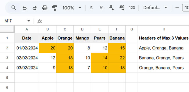
To get the headers of the top 3 values in each row, use the following formula in cell H2 and drag it down:

=TEXTJOIN(", ", TRUE, UNIQUE(MAP(SORTN(TOCOL(B2:F2, 0), 3, 0, 1, FALSE), LAMBDA(r_, IFNA(FILTER($B$1:$F$1, B2:F2=r_, B2:F2>0))))))

Where:

• $B$1:$F$1 is the header row reference.
• B2:F2 is the range of quantities.
• 3 in SORTN(..., 3, 0, 1, FALSE) determines the number of maximum values to return.

When you drag the formula down, the header row reference remains the same (due to absolute referencing), while the quantity row reference adjusts for each row. This allows the formula to return the headers of the top 3 values for each row.

How the Formula Works:

• TOCOL(B2:F2 , 0): Converts the row values into a column and removes empty cells.
• SORTN(..., 3, 0, 1, FALSE): Sorts the values in descending order and returns the top 3 values.
• MAP(..., LAMBDA(r_, IFNA(FILTER($B$1:$F$1, B2:F2=r_, B2:F2>0)))):
  • Filters the headers where the quantity matches the current value in the SORTN result and is greater than 0.
  • The MAP function applies this logic to each value in the SORTN result.
• UNIQUE(...): Removes duplicate headers corresponding to multiple occurrences of the same maximum value.
• TEXTJOIN(", ", TRUE, ...): Combines the headers into a single cell, separated by commas.

This is how the formula finds the headers of the top N values in a row.

Array Formula

If you don’t want to drag the formula down and instead want it to automatically expand, use the BYROW function to apply the formula to each row in the range:

=BYROW(B2:F, LAMBDA(er_, TEXTJOIN(", ", TRUE, UNIQUE(MAP(SORTN(TOCOL(er_, 0), 3, 0, 1, FALSE), LAMBDA(r_, IFNA(FILTER(B1:F1, er_=r_, er_>0))))))))

Here, the drag-down formula is converted into a custom LAMBDA function:

LAMBDA(er_, TEXTJOIN(", ", TRUE, UNIQUE(MAP(SORTN(TOCOL(er_, 0), 3, 0, 1, FALSE), LAMBDA(r_, IFNA(FILTER(B1:F1, er_=r_, er_>0)))))))

The BYROW function applies this lambda function to each row in the range B2:F.

Find Unique Max N Values in a Row and Return Their Headers

Using the same sample data, here’s the drag-down formula to find the headers of the unique top 3 values. Place it in cell H2:

=TEXTJOIN(" | ", TRUE, MAP(SORTN(TOCOL(B2:F2, 0), 3, 2, 1, FALSE), LAMBDA(r_, TEXTJOIN(", ", TRUE, IFNA(FILTER($B$1:$F$1, B2:F2=r_, B2:F2>0))))))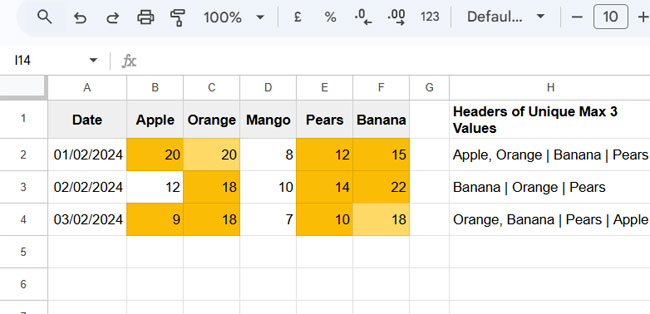

Where:

• $B$1:$F$1 is the header row reference.
• B2:F2 is the row reference containing the quantities.
• 3 in SORTN(..., 3, 2, 1, FALSE) determines the number of unique maximum values to return.

This formula displays the results in a user-friendly format:

• Headers corresponding to the same maximum value are comma-separated.
• Headers corresponding to different maximum values are pipe-separated.

For example:

Apple, Orange | Banana | Pears

• Apple and Orange correspond to the first maximum value.
• Banana corresponds to the second maximum value.
• Pears corresponds to the third maximum value.

How the Formula Works:

• TOCOL(B2:F2 , 0): Converts the row values into a column and removes empty cells.
• SORTN(..., 3, 2, 1, FALSE): Sorts the values in descending order, removes duplicates, and returns the top 3 unique values.
• MAP(..., LAMBDA(r_, TEXTJOIN(", ", TRUE, IFNA(FILTER($B$1:$F$1, B2:F2=r_, B2:F2>0))))):
  • Filters the headers where the quantity matches the current value in the SORTN result and is greater than 0.
  • Combines multiple headers (if any) into a single cell, separated by commas.
• TEXTJOIN(" | ", TRUE, ...): Combines the results for each unique maximum value into a single cell, separated by pipes.

Array Formula for Unique Max N Values

To avoid dragging the formula down, use the BYROW function to create an array formula:

=BYROW(B2:F, LAMBDA(er_, TEXTJOIN(" | ", TRUE, MAP(SORTN(TOCOL(er_, 0), 3, 2, 1, FALSE), LAMBDA(r_, TEXTJOIN(", ", TRUE, IFNA(FILTER(B1:F1, er_=r_, er_>0))))))))

This formula applies the same logic as the drag-down version but automatically processes each row in the range B2:F.

Resources

• Find the Column Header of the Max Value in Google Sheets
• Lookup and Retrieve Column Headers in Google Sheets
• Search Across Columns and Return the Header in Google Sheets
• How to Retrieve Column Header of Min Value in Google Sheets
• Get the Headers of the First Non-Blank Cell in Each Row in Google Sheets
• Get the Header of the Last Non-Blank Cell in a Row in Google Sheets