The easiest way to filter the last N days of data in Google Sheets is by using the FILTER function in combination with the ISBETWEEN function. Additionally, you may need to use the TODAY and MAX functions, depending on your specific use case.

Below, you will find three formulas, each handling a different scenario. These formulas filter the last N days of data based on:

1. Today’s date (rolling window approach)
2. A user-defined date
3. The maximum date in the dataset

Sample Data

The sample dataset consists of:

• Column A: Dates
• Column B: Items (fruit names)
• Column C: Quantities

The filtering range is A2:C, excluding the header row.

Filter Last N Days from Today (Rolling Window Approach)

The following formula filters the last 7 days of data from today:

=FILTER(A2:C, ISBETWEEN(A2:A, TODAY()-7, TODAY()-1))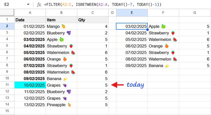

Formula Explanation:

• A2:C is the range to filter.
• ISBETWEEN(A2:A, TODAY()-7, TODAY()-1) is the condition.
• The formula filters rows where the condition is TRUE.
• The ISBETWEEN function checks if each date in A2:A falls between TODAY()-7 and TODAY()-1.

This formula excludes today’s date. If you want to include today, modify it as follows:

=FILTER(A2:C, ISBETWEEN(A2:A, TODAY()-6, TODAY()))

Filter Last N Days from a Specific Date (User-Defined Date)

The formula above dynamically adjusts based on TODAY(), making it a rolling window approach. However, you might need to filter data relative to a specific date instead.

To do this, replace TODAY() with a user-defined date using the DATE(year, month, day) function. For example, to filter the last 7 days from 12/02/2025:

=FILTER(A2:C, ISBETWEEN(A2:A, DATE(2025, 2, 12)-7, DATE(2025, 2, 12)-1))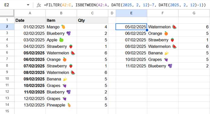

Key Notes:

• This formula filters data for the last 7 days relative to 12/02/2025.
• The filtered data excludes 12/02/2025. To include it, modify the formula as follows:

=FILTER(A2:C, ISBETWEEN(A2:A, DATE(2025, 2, 12)-6, DATE(2025, 2, 12)))

This formula is useful for historical data analysis.

Filter Last N Days from the Latest Date in the Data

In cases where your dataset is irregularly updated, you may not have today’s date or a specific reference date. Instead, you can filter data based on the latest date in your dataset using the MAX function.

Here’s how:

=FILTER(A2:C, ISBETWEEN(A2:A, MAX(A2:A)-7, MAX(A2:A)-1))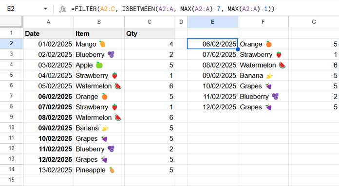

Formula Explanation:

• MAX(A2:A) finds the latest date in column A.
• The formula then filters the last 7 days from this latest date.

This excludes the latest date. To include it, modify the formula as follows:

=FILTER(A2:C, ISBETWEEN(A2:A, MAX(A2:A)-6, MAX(A2:A)))

This approach is ideal for datasets that are updated at irregular intervals.

Resources

• How to Find a Specific Previous Day from a Date in Google Sheets
• Google Sheets Query to Extract All the Rows from Previous Month
• Current Quarter and Previous Quarter Calculation in Google Sheets
• Get Last 7, 30, and 60 Days Total in Each Row (from Today) in Google Sheets
• How to Highlight the Latest N Values in Google Sheets
• Filter or Find Current Week This Year and Last Year in Google Sheets
• Formula to Conditionally Filter Last N Rows in Google Sheets
• Filter Data for a Specific Number of Past Weeks in Google Sheets
• Filter Data by Week (This, Last, or N Weeks Ago) – Google Sheets
• How to Filter Current Week Horizontally in Google Sheets