")
")


")


")

")
")
 in Excel & Google Sheets")


How do I filter out rows where all cells — or, in other words, the entire row — are blank in Google Sheets? I don’t want to use any helper columns for this.
Usually, we decide a row is blank if the first cell in that row is blank, because most of the time, the first column in a table contains timestamps or IDs.
But in this case, we don’t want to follow that method. We want to check if any cell in a row has a value — and if so, return that row.
For example, I have a sample table filled with my birding data in Google Sheets.
The fields are: “Scientific Name,” “Common Name,” “Locale,” “State,” “Country,” “Number of Occurrences,” and “Date.”
The range is A1:G.
We want to filter out rows where the entire row is blank.
Of course, we can use either the FILTER function or the Filter menu to do that.
When using the FILTER function, there are two approaches: In the condition part of the formula, you can either use a LAMBDA formula or a QUERY formula.
Filter Out If All Cells in a Row Are Blank: QUERY Approach
Here is my sample birding data:
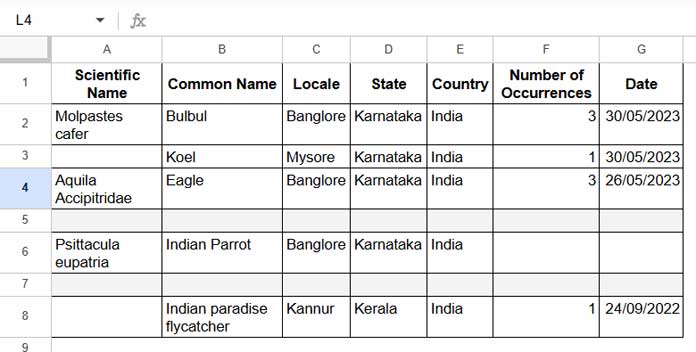
In this table, there are two fully blank rows — A5:G5 and A7:G7.
We can use the following FILTER formula in cell I1:
=FILTER(A1:G, LEN(TRIM(TRANSPOSE(QUERY(TRANSPOSE(A1:G),,9^9)))))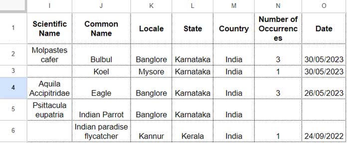
How Does It Work (Especially the QUERY Part)?
In the above formula, QUERY is used to join columns dynamically so we can check — using LEN — whether the combined row has any value.
It works like this:
- QUERY Syntax:
QUERY(data, query, [headers]) - data:
TRANSPOSE(A1:G) - query: (nil — left empty)
- headers:
9^9
By specifying 9^9 (an arbitrarily large number) for the headers argument, we tell QUERY that all rows are headers. As a result, QUERY combines them into a single row.
We must use transposed data; otherwise, QUERY would combine values column-wise instead of row-wise.
(You can try using =QUERY(A1:G9,,9^9) directly in your Sheet to observe how it works.)
Filter Out If All Cells in a Row Are Blank: LAMBDA Approach
Alternatively, we can use the BYROW function to process each row individually:
=FILTER(A1:G, LEN(BYROW(A1:G, LAMBDA(row, TEXTJOIN("", TRUE, row)))))How It Works:
- BYROW processes each row of the range.
- Inside the LAMBDA, TEXTJOIN combines all cells in the row into a single text string.
- LEN returns the length of that string — if it’s greater than 0, the row contains data.
- Finally, FILTER keeps only those rows where the length is greater than 0.
This is another efficient way to filter out rows where all cells are blank.
How to Do This Using the Filter Menu
You can also use the Filter menu to filter out empty rows without writing a formula.
Here’s how:
- Select the range (e.g.,
A1:G). - Click Data > Create a filter.
- Click the filter drop-down in cell
A1and choose Filter by condition > Custom formula is. - Enter the custom formula:
- To show non-blank rows:
=COUNTIF($A2:$G2, "<>")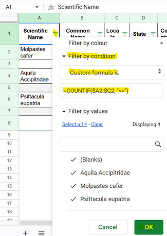
- To show only blank rows:
=COUNTIF($A2:$G2, "<>")=0
- To show non-blank rows:
- Click OK.
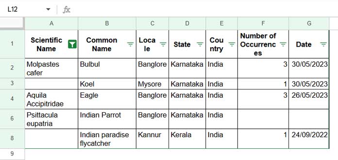
This method lets you easily view only the rows that are fully blank or those that contain at least one value.