There is no direct way to filter as you type in Google Sheets. However, you can use a workaround that is quite effective, though not 100% perfect. In Excel, you may have seen people filtering a table dynamically as they start typing in a search field.

To filter as you type, you need to capture the value of the search field in real time in another cell. This value can then be used in a FILTER formula.

Unfortunately, this is not natively possible in Google Sheets, so we have to rely on a workaround.

Workaround for Filtering As You Type in Google Sheets

In Excel, the Combo Box (ActiveX Control) can be used as a search field that transfers the entered value to another cell in real-time.

However, Google Sheets does not have an equivalent Combo Box feature. Instead, we can use a different approach to achieve a similar result.

Source Data

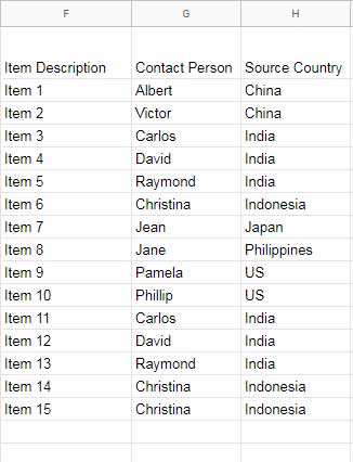
For this example, we will filter rows based on the Source Country column. You can easily modify it to filter based on another column later.

Sample Sheet

Steps to Filter As You Type in Google Sheets

Since Google Sheets does not have a built-in Combo Box like Excel, we need an alternative.

Fortunately, Google Sheets’ drop-down list feature (Insert > Drop-down > Drop-down from a range) offers real-time search suggestions.

Search Suggestion Feature in Google Sheets

One interesting characteristic of this feature is that it suggests words based on the first letter of any word in a phrase within a cell.

For example, typing the letter “e” will suggest all items containing “East,” even if it’s the second word in the phrase. We can leverage this behavior to create our live filter.

However, this method does not perform real-time filtering. Instead, it provides search suggestions in real-time, and the actual filtering happens when you press Enter or select a suggestion.

1. How to Create a Search Suggestion Drop-Down in Google Sheets

Since our data spans multiple rows and three columns, we first need to combine the values from these columns into a single column. This will serve as the source for our drop-down search suggestion.

If your sample data is in F1:H16, enter the following formula in I2:

=ArrayFormula(F2:F16&REPT(".", 10)&G2:G16&REPT(".", 10)&H2:H16)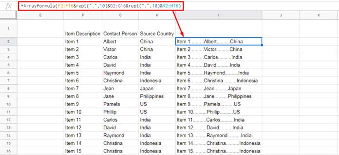

If your list grows dynamically, use this version instead:

=ArrayFormula(IF(LEN(F2:F), F2:F&REPT(".", 10)&G2:G&REPT(".", 10)&H2:H,))

This formula joins values from columns F, G, and H, separating them with ten dots (.) for better readability in the drop-down list.

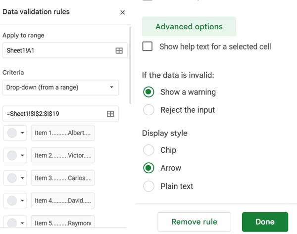
2. Setting Up the Drop-Down Search Field

1. Merge cells A1:C1 (Format > Merge Cells > Merge All).
2. Click Insert > Drop-down, and select Drop-down (from a range) under Criteria.
3. Under Advanced options, ensure that “Show a warning” is selected instead of “Reject the input.”
4. Click Done.

Now, when you type in the search field (merged cell A1:C1), matching suggestions will appear.

3. Filter Formula to Extract Rows Based on Search Suggestion

The FILTER function in Google Sheets does not support wildcards directly. To filter column H based on partial matches, we can use REGEXMATCH within FILTER.

Applying the Filter Formula

Enter this formula in A3:

=IFERROR({F1:H1; FILTER(F2:H, REGEXMATCH(H2:H, "^(?i)"&A1))})

How It Works:

• REGEXMATCH(H2:H, "^(?i)"&A1): Checks if the search key in A1 matches any value in column H (case insensitive).
• FILTER(F2:H, REGEXMATCH(...)): Extracts matching rows.

This method provides a workaround to filter rows dynamically as you type in Google Sheets.

Changing the Filter Column

Since the drop-down search suggestion works based on the first letter of any word, you can easily change the filtering column.

To filter based on Item Description (column F) instead of Source Country (column H), update the formula in A3 as follows:

=IFERROR({F1:H1; FILTER(F2:H, REGEXMATCH(F2:F, "^(?i)"&A1))})

Conclusion

While Google Sheets does not support filter as you type in Google Sheets natively, this workaround using drop-down search suggestions and the FILTER function provides a practical solution. Although it does not filter in real-time, it enables quick searching and filtering upon selection.

Additional Resources

• How to Create a Search Box Using QUERY in Google Sheets
• How to Create a Simple Multi-Column Search Box in Google Sheets
• Google Sheets: How to Get an “All” Selection Option in a Drop-down
• Create a Drop-Down to Filter Data From Rows and Columns
• Multi-Row Dynamic Dependent Drop-Down List in Google Sheets
• Auto Populate Information Based on Drop-Down Selection in Google Sheets