How to Create a Search Box with QUERY in Google Sheets

You can create a custom search box in Google Sheets to extract rows that match the search phrase in a column.

We will use the QUERY function for this purpose, as it is one of the best functions for filtering rows based on substring matches in Google Sheets.

It helps apply filters to a column by partially matching text strings, such as those that start with a specific word, end with a specific word, contain specific words, match wildcards, or follow a pattern.

In essence, the search box acts as an advanced filtering tool with various options for filtering.

Functionality of a QUERY-Powered Search Box in Google Sheets

The ultimate goal is to filter a large set of data based on string comparisons, though the purpose may vary from person to person.

I use the search box in Google Sheets for the following purposes:

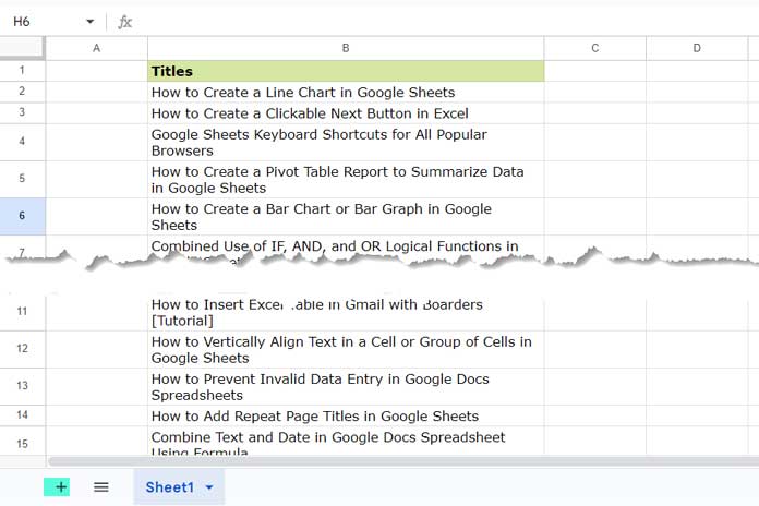
I have over a thousand Google Sheets tutorials on this blog. I’ve copied the titles of all these tutorials into a column in Google Sheets.

As a side note, if you have fewer than 250 blog posts, you can use the IMPORTFEED function to import the titles into Google Sheets.

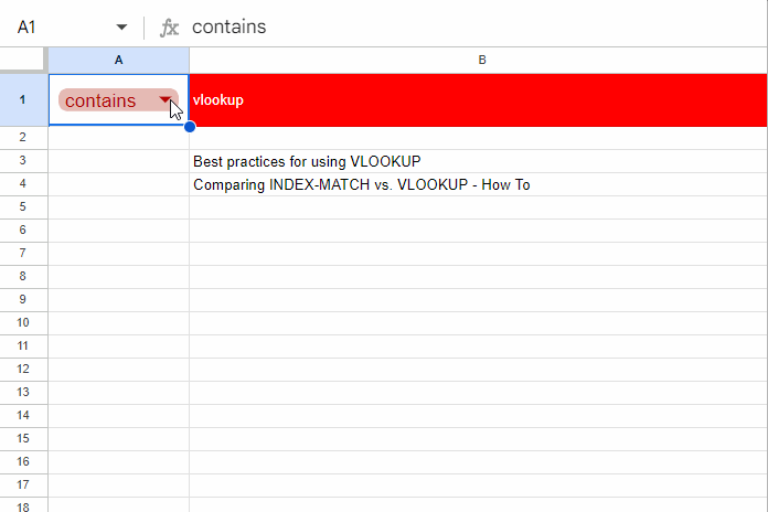
My goal is to verify that I haven’t already written a tutorial on a specific topic before starting a new one. For example, I have several tutorials on the keyword ‘vlookup’ that address different problems with this function.

I can use the search box to filter the titles that match “vlookup” and ensure that the topic isn’t already covered.

Using my custom search box in Google Sheets, I can search for keywords in various ways. I am making the best use of QUERY’s string comparison operators in the custom search box that I’ve created.

Download Search Box Template

If you want to learn how to create a search box using QUERY in Google Sheets, just keep reading.

There are five steps involved:

Preparing the sample data for the search
Preparing the Search Box Field
Setting data validation in the search field to allow only lowercase letters
Adding drop-down chips to control the level of string comparison and filtering
Using the QUERY formula to power the search

Let’s go through these steps one by one to create a powerful search box in Google Sheets.

Step 1: Preparing the Data

Create a new Google Sheets file by clicking Sheets.new.

In this file, enter, import, or copy-paste the data you want to search using a keyword into column B.

Use cell B1 for the field label and enter your data below it.

Preparing Data for Search in Google Sheets

We will create the search box on a second sheet in that file.

To do this, click the + button at the bottom left (refer to the screenshot above, where the button is highlighted in cyan). This will create Sheet2.

Navigate to Sheet2 and click on column letter B to select the column.

Hover your cursor over the right edge of the column header until the hand icon changes to a double-headed arrow.

Click and drag the edge to adjust the column width to your desired size.

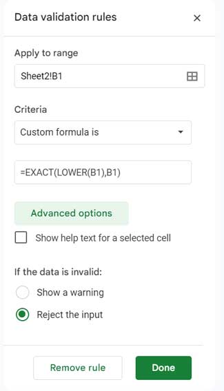
Step 3: Validating Keyword Entry

Cell B1 will be your search field where you will enter the keyword. Since the QUERY function is case-sensitive, we need to ensure that only lowercase letters are allowed in this cell to avoid case-sensitivity issues.

Navigate to cell B1 in Sheet2.
Click on Data > Data validation to open the Data Validation panel on the sidebar.
Click Add rule.
Under Criteria, select Custom formula is.
Enter the following formula in the field below: =EXACT(LOWER(B1), B1).
Under Advanced options, check Reject input.
Click Done to close the panel.

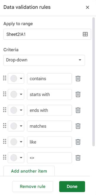
Data Validation to Enforce Lowercase Text Entry

Step 4: Create a Drop-down to Select a String Comparison Option

In this step, we will create a drop-down box in cell A1 on Sheet2 with the following options:

contains
starts with
ends with
matches
like
<>

These options are string comparison operators that control how the output is filtered based on the keyword entered in the search box in cell B1.

Navigate to cell A1 on Sheet2.
Click Insert > Drop-down.
In the sidebar panel, replace “Option 1” with “contains,” and “Option 2” with “starts with.”
Click Add another item and enter “ends with,” then enter the remaining options similarly.
Once all items are added, click Done.

Drop-down Menu to Select String Comparison Operators for Keyword Searching in the Search Box

We have completed the setup of the search box. The next step is to apply the QUERY formula.

Use this QUERY formula in cell B3:

=IFERROR(IF(LEN(B1), QUERY(Sheet1!B2:B, "Select B where lower(B) "&A1&" '"&lower(B1)&"'"), "Not found!"))

That’s it! Your custom search box in Google Sheets is ready. Type your search phrase in cell B1, and then select one of the comparison operators in cell A1. I recommend selecting “contains” in cell A1, as it will cover most use cases.

Here are a few examples of how to use the search box in Google Sheets:

Assume the keyword is “how to”. Enter it in cell B1.
In cell A1, select one of the string comparison operators:
- contains: Returns all rows that contain the string “how to” in Sheet1!B2:B.
- starts with: Returns all rows that start with the text “how to”.
- ends with: Returns all rows that end with the text “how to”.
- <>: Returns rows that do not match the keyword in cell B1. This is a full match, not a partial match.
- like: Allows you to use wildcards. % acts like * (matches any sequence of characters), and _ acts like ? (matches a single character). For example, entering %vlookup% in cell B1 returns all rows that partially match “vlookup” (similar to “contains”). Entering _lookup% will return rows that start with “vlookup,” “xlookup,” “hlookup,” etc.
- matches: Uses regular expressions (regex) for matching. This requires knowledge of regular expressions, which you can learn about in my relevant tutorial.

Resources

21 COMMENTS

Ben M January 27, 2021 At 12:27 am

Hi Prashanth,

I have a google sheet with all of the seeds I have for the next gardening season. I want to be able to search for a name and then have it display all of the information within that row.

So if I Vlookup up “Tomato”, A listing of each row where the title (column1) at least contains the word “Tomato” and what comes up is everything within that row (in each column) with header titles proceeding each new column. Ie:

Roma Tomato, Sunlight: Full Sun, Days to Maturity: 80 Days
Plum Tomato, Sunlight: Partial Sun, Days to Maturity: 45 Days

Thanks!

- Prashanth January 27, 2021 At 4:40 pm
  
  Hi, Ben M,
  
  Here is an example.
  
  Assume the table contains 3 columns (A1:C) and column A contains the name of seeds.
  
  So, you can use the below Query.
  
  =query(A1:C,"Select * where A contains 'Tomato'")
  
  In this, the criterion is “Tomato”. Enter this criterion (without double quotes) in cell E1. Then the formula would be;
  
  =query(A1:C,"Select * where A contains '"&E1&"'")
  
Donna Osmon January 27, 2021 At 12:22 am

I’m using Google sheets to maintain a list of addresses that we’ve collected items from, where we limit them to 3 per year.

I’m new to Sheets so I’m not sure how to even begin. What formula would I use to search by house number, followed by Street name?

- Prashanth January 27, 2021 At 4:05 pm
  
  Hi, Donna Osmon,
  
  Make a sheet that contains some sample addresses and share that sheet link via a reply to this comment.
  
  I would be happy to assist.
  
Frank December 8, 2020 At 2:12 am

What would be the simplest way of having no queried values displayed if nothing is entered into B1?

i.e. I do not want a list of thousands of values displayed when B1 is empty.

- Prashanth December 8, 2020 At 8:41 am
  
  Hi, Frank,
  
  You may please modify the formula as below.
  
  =iferror(if(B1="",,query(Links!A2:A,"Select A where lower(A) "&A2&" '"&B1&"'")),"Not found!")
  
babop September 19, 2020 At 12:47 am

This is just what I was looking for – thank you.

Is it possible to display the result in the cell below the formula so I can copy and paste it?

- Prashanth September 19, 2020 At 10:38 am
  
  Hi, babop,
  
  This will add one blank row on the top.
  
  ={"";iferror(if(len(B1),query(Links!B2:B,"Select B where lower(B) "&A1&" '"&lower(B1)&"'"),"Not found!"))}
  
  But actually adding one row on the top is not required to copy-paste the result.
  
  It doesn’t matter whether there is a blank row on the top or not, you must copy and paste it as values (copy, right click to see “paste special”).
  
Ervin May 2, 2020 At 9:10 am

Hi there,

I have a phone book where each letter has its own sheet from a-z, how can I make this formula work so that when I want to find everyone living in a certain street I can search “contains the street name” and it shows all the names that live in that street? Thank you.

- Prashanth May 2, 2020 At 3:16 pm
  
  Hi, Ervin,
  
  You may need to import the data from the sheets A-Z in a master sheet. Then you can use my formula.
  
  To import data from the sheets A to Z to a master sheet, you can use the syntax as per the formula below.
  
  =query({A!A1:B;B!A1:B;'C'!A1:B},"Select * where Col1 is not null")
  
  This formula will import data from Sheet A, B, and C to a master sheet. The columns included are columns A and B.
  
  Once imported (compiled) the data, you can try the search box explained in this guide (multi-column search).
  
  Filter Rows if Search Key Present in Any Cell in that Rows in Google Sheets.
  
Sarah Daly January 20, 2020 At 4:59 pm

Hi there,

How would I go about searching across multiple sheets?

- Prashanth January 21, 2020 At 9:07 am
  
  Hi, Sarah Daly,
  
  Include the sheets within the formula. Here I am including the sheets Sheet1, Sheet2, and Sheet3.
  
  =iferror(query({'Sheet1'!A2:A;'Sheet2'!A2:A;'Sheet3'!A2:A},"Select Col1 where lower(Col1) "&A2&" '"&B1&"'"),"Not found!")
  
  Please note the changes.
  
Seth October 18, 2019 At 4:08 am

How can I make this search box using Query work for a mixture of numbers and words?

For example, if one cell contained “222′ and the cell below that contained “Fun”.

At the moment, whenever a value is entered into the Links list on your example sheet the formula hits the error “Not Found” message.

- Prashanth October 18, 2019 At 9:45 am
  
  Good question.
  
  Use To_text with the data (range) and change Colum identifiers from A to Col1.
  
  Formula:
  
  =ArrayFormula(iferror(query(to_text(Links!A2:A),"Select Col1 where lower(Col1) "&A2&" '"&B1&"'"),"Not found!"))
  
  Here is a related post – How to Solve the Mixed Data Type Issue in Query in Google Sheets.
  
Ram October 4, 2019 At 3:01 pm

Hi, I followed the steps above. When I enter the formula in cell B2, all values are returned in B2 and cell B1 not working. Am I missing anything?

- Prashanth October 4, 2019 At 9:36 pm
  
  Hi, Ram,
  
  Did you see my example Sheet linked within the post?
  
  You can refer to that to sort out the error.
  
  Best,
  
Chris September 20, 2019 At 9:14 pm

If you add into LOWER() into the B2 formula by using the formula:

=iferror(query(Sheet1!A2:A,"Select A where lower(A) "&A2&" '"&LOWER(B1)&"'"),"Not found!")

Then you skip on needing any data validation within B1. People can enter anything and the search is not case sensitive.

Nikki Alvs September 2, 2019 At 3:21 pm

Hello!

What if I want to hide my source file. Can I use Importrange? How do I make it work with this formula?

Thank you!

- Prashanth September 3, 2019 At 8:38 am
  
  Hi, Nikki,
  
  To hide your source file that contains the information to search, as you have said, you can use the Importrange.
  
  See the changes in the formula below.
  
  =iferror(query(importrange("Your File URL here","'your tab name'!A1:A"),"Select Col1 where lower(Col1) "&A2&" '"&B1&"'"),"Not found!")
  
  Note: First enter the Importrange formula alone and ‘Allow access’. Delete it. Then use the above formula.
  
  Best,
  
Gabriel Cerqueira August 3, 2019 At 6:00 pm

Hello. What if you want to search something giving 2 columns? for example, select A, B where lower(A), lower(B) contains…

- Prashanth August 4, 2019 At 10:20 am
  
  Hi, Gabriel Cerqueira,
  
  Here is one example.
  
  =Query(A1:B,"Select A,B where lower(A) contains 'apple'and lower(B) contains 'apple'")
  
  Best,