We can extract time from DateTime (timestamp) in many ways in Google Sheets and here are the 3 most effective methods.

This will be useful when extracting current time that recalculates or a static time component from a timestamp.

What’s a Timestamp or DateTime in Google Sheets?

A timestamp or DateTime in Google Sheets represents a specific point in time, including both the date and the time.

You can get a timestamp using connected forms, function combinations, manual entry, or the NOW function.

To enter the date “2024-06-25” and time “10:10:10” together in cell A1, you can type “2024-06-25 10:10:10” into the cell. This is in the ISO 8601 format, an international standard for representing date and time.

Depending on your Google Sheets’ default format, you might see it displayed in the formula bar as “DD/MM/YYYY HH:MM:SS” or “MM/DD/YYYY HH:MM:SS.”

If you want, you can apply that format by going to Format > Number > Custom Date and Time.

If you want to use the above timestamp as a criterion, specify it as “2024-06-25 10:10:10” or use the formula DATE(2024, 6, 25) + TIME(10, 10, 10), where the date is as per the syntax DATE(year, month, day) and the time is as per the syntax TIME(hour, minute, second).

Examples:

=COUNTIF(A2:A, DATE(2024, 6, 25) + TIME(10, 10, 10))
=COUNTIF(A2:A, "2024-06-25 10:10:10")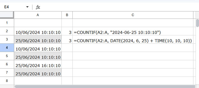

These COUNTIF formulas count the occurrences of the DateTime “2024-06-25 10:10:10” in cells A2:A.

Extracting Static Time from DateTime in Google Sheets

Assume the range A2:A10 contains static timestamps. These timestamps may be imported, fed by a Google Forms form, or hand-entered.

In that case, you can use the following formulas to extract the time from these timestamps.

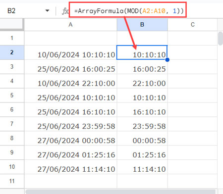
Method 1: Using the MOD Function

Enter the following formula in cell B2 and drag the fill handle down to B10:

=MOD(A2, 1)

Or you can enter it as an array formula in cell B2 to spill the results down:

=ArrayFormula(MOD(A2:A10, 1))

The formula will return the result in DateTime format. For example, if the DateTime is “2024-06-10 10:10:10”, the formula will return “30/12/1899 10:10:10”. The serial number of 30/12/1899 is equal to 0.

You can select B2:B10 and apply Format > Number > Time to get the time in the proper format.

Formula Breakdown:

The MOD function returns the remainder of a division operation. The syntax is:

MOD(dividend, divisor)

DateTime values in Google Sheets are stored as numbers, where the integer part represents the date, and the fractional part represents the time.

When the ‘divisor’ is 1, the remainder will be the fractional part of the number, which corresponds to the time portion.

This is my preferred method to extract time from DateTime in Google Sheets.

Method 2: Using the INT Function

Similar to the MOD function, you can use the INT function to extract the time portion from DateTime values for the range A2:A10.

Non-Array Formula for cell A2:

=A2-INT(A2)

Array Formula for the range A2:A10:

=ArrayFormula(A2:A10-INT(A2:A10))

The output will be in DateTime format. To display the result as time, you can apply Format > Number > Time to the result range.

Formula Breakdown:

The INT function returns the integer part of a number by rounding down to the nearest integer. The syntax is:

INT(number)

Since DateTime is stored as a serial number, where the integer part represents the date, you can extract the fractional part (which represents the time component) by subtracting the integer part from the DateTime value.

This method efficiently isolates the time component from DateTime values in Google Sheets.

Method 3: Using the TEXT Function

In this method, we utilize the TEXT function either alone or in combination with the TIMEVALUE function to extract the time component.

Using TEXT Function Alone:

When using the TEXT function alone, it doesn’t directly extract the time component but formats the timestamp to display the time as text output.

Example:

=TEXT(A2,"HH:MM:SS")

This will also work with an array formula:

=ArrayFormula(TEXT(A2:A10,"HH:MM:SS"))

Unlike the other two methods, this doesn’t require formatting the result to time.

Using TEXT and TIMEVALUE Combo:

By combining TEXT and TIMEVALUE (which converts a time string to time values), you can effectively extract time from DateTime values as follows:

Formula:

=TIMEVALUE(TEXT(A2,"HH:MM:SS"))
=ArrayFormula(TIMEVALUE(TEXT(A2:A10,"HH:MM:SS")))

The result will be time values represented as fractional numbers. To display them properly as time, select the result range and apply Format > Number > Time.

Get Current Time in Google Sheets

The NOW function returns the current DateTime in Google Sheets.

To extract the current time from the DateTime, you have several options:

MOD Function:

=MOD(NOW(), 1)

INT Function:

=NOW()-INT(NOW())

TEXT Function (in text format):

=TEXT(NOW(), "HH:MM:SS")

Using TEXT and TIMEVALUE Combo (as time values):

=TIMEVALUE(TEXT(NOW(), "HH:MM:SS"))

If you use the first two formulas or the fourth formula, which is an extended version of the third formula, you should format the result to time.

These formulas will help you extract the current time in Google Sheets.

Resources

Here are some Google Sheets resources that discuss using timestamps.

• How to Insert a Static Timestamp in Google Sheets
• Convert Unix Timestamp to Local DateTime and Vice Versa in Google Sheets
• Extract the Earliest or Latest Record in Each Category Based on Timestamp
• How to Compare Timestamp with Normal Date in Google Sheets
• How to Filter Timestamp in Query in Google Sheets
• How to Use Timestamp within IF Logical Function in Google Sheets
• Vlookup Date in Timestamp Column in Google Sheets
• How to Remove Milliseconds from Timestamps in Google Sheets
• How to Hardcode DATETIME Criteria within FILTER Function in Google Sheets
• Extracting Date From Timestamp in Google Sheets: 5 Methods
• How to Use DateTime in Query in Google Sheets
• How to Convert a Timestamp to Milliseconds in Google Sheets
• How to Increment DateTime by One Hour in Google Sheets (Array Formula)