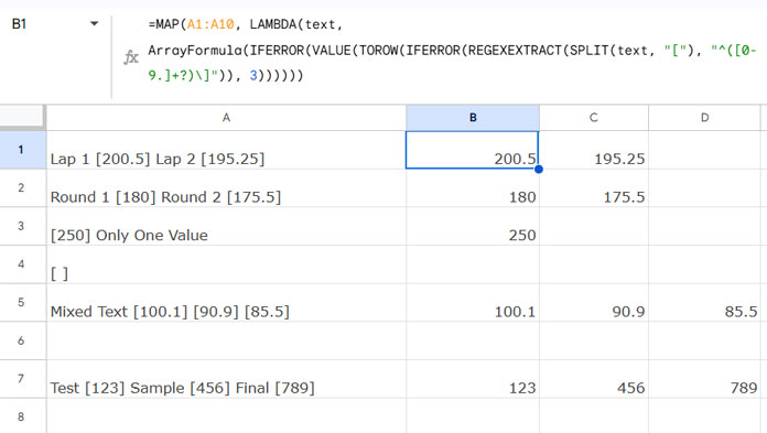
Extract Numbers Within Square Brackets in Each Row in Google Sheets

I have sentences/phrases in each row in a column that may or may not contain multiple square brackets. Within that available square brackets, there may be numbers. How to extract numbers within square brackets in each row in Google Sheets. That’s what I am going to detail in this Google Docs Sheets tutorial.

To extract numbers within a single square bracket in a cell you can use the below RegexExtract formula.

Value in cell B1: Team A [200]

=iferror(REGEXEXTRACT(B1, "\[(.+)]"))

Result: 200

Array Formula to Extract Numbers Within Square Brackets

If there are multiple values in a range like B1:B, no doubt, you can convert the above formula as an Array Formula.

=ArrayFormula(iferror(REGEXEXTRACT(B1:B, "\[(.+)]")))
Array Formula to Extract Numbers Within Square Brackets

You can sue the above Regexextract formula to extract numbers within square brackets in each row in Sheets. But what about extracting numbers within multiple square brackets in the same cell?

No doubt, the above formula would fail miserably! Here comes the relevance of this tutorial.

Extract Numbers Within Multiple Square Brackets in Each Row

Sample Data and the Result Expected:

Extract Numbers Within Multiple Square Brackets

See the above sample data (B2:B) with numbers in multiple square brackets in each row.

The output is spread across the range C2:E. If you want you can get the total of the values in square brackets in each row using an MMULT formula later. First of all, let me elaborate on how to get the same above output.

Steps to Extract Numbers Within Multiple Square Brackets

Just follow the below step-by-step instructions. I will take you thru’ each and every step to create a combo formula that extracts multiple values from square brackets.

Step 1: Filter out blank rows at the end of the source data range.

=filter(B2:B,B2:B<>"")

While using the above Filter formula, please make sure that you are not leaving any blank cells in between. I mean as per the current range B2:B, there should not be any blank cells in the range B2:B5.

Step 2: Split the Text Strings Using “[” as the delimiter.

Here in the below Split formula, the range (the texts to split by delimiter) is the above Filter formula.

=ArrayFormula(split(filter(B2:B,B2:B<>""),"["))
Split using opening square bracket as the delimiter

Step 3: Extract the Numbers with Closing Square Brackets.

Here we can use the ‘same’ RegexExtract formula that I have used in the beginning. But wait!

In the split, I have used the opening square bracket as the delimiter. As a result, the split output is missing the same.

At the beginning of this tutorial, I have used this "[(.+)]" regular expression to extract numbers within a single open and close square bracket.

Since the absence of the opening square bracket, we must modify this regular expression this time. See that below.

First, we can use the range D2:F5 (please refer the above image). Then we can replace this range with the formula in cell D2 itself.

=ArrayFormula(iferror(REGEXEXTRACT(D2:F5, "(.+)]")))

Here I am replacing D2:F5 with the relevant formula which I have keyed in cell D2 earlier.

=ArrayFormula(iferror(REGEXEXTRACT(split(filter(B2:B,B2:B<>""),"["), "(.+)]")))
Combo formula to extract numbers from multiple square brackets

This way you can extract numbers within multiple square brackets in Google Sheets. But this is not our final formula. Why?

See the output. The extracted numbers are formatted as text (left aligned). This is due to the use of the RegexExtract function, which is text.

Final Formula:

Multiply the above output with the number 1 to make the numbers numeric. Also, this will place 0 values in blank cells. This is required if you want to sum the extracted values in each row using the MMULT function.

=ArrayFormula(iferror(REGEXEXTRACT(split(filter(B2:B,B2:B<>""),"["), "(.+)]"))*1)
Take numbers outside of square brackets in Google Sheets

How to Sum the Extracted Numbers in Each Row in Google Sheets

This is an additional tip. By using MMULT, you can very easily sum the above values in each row.

Take the last formula (formula output) as the Maxtrix 1 in MMULT.

Syntax:

MMULT(matrix1, matrix2)

Since there are 3 columns in the above output, create a 3 row virtual array as below to use as Matrix 2.

={1;1;1}

I am not going in to the logic. Here is that MMULT formula.

=MMULT(ArrayFormula(iferror(REGEXEXTRACT(split(filter(B2:B,B2:B<>""),"["), "(.+)]"))*1),{1;1;1})
Extract and Sum numbers within brackets in each row

The above formula is not flexible due to the use of virtual array (Matrix 2). Instead of using;

={1;1;1}

We can use the below ROW formula. Both are equivalent.

=ArrayFormula(row(A1:A3)^0)

Even if you use the Row formula as matrix 2, we can not say the MMULT above is dynamic. Because of matrix 2 which is some kind of manual formula.

In matrix 2, what we want is a virtual array. In that, the number of rows (each row contains the value 1) must be equal to the number of columns in the “Final formula”.

There are 3 columns in the “final formula”. That’s why I have generated a virtual column with three rows.

But the number of columns in the “final formula” may vary depending on the data in B2:B.

So in the just above Row formula, we may find a way to replace the A3 with A’n’. How to find the ‘n’ then?

Wrap the “final formula” with the COLUMNS function. It would return the number of columns dynamically.

=columns(ArrayFormula(iferror(REGEXEXTRACT(split(filter(B2:B,B2:B<>""),"["), "(.+)]"))*1))

Modify the Row formula as below.

From this;

=ArrayFormula(row(A1:A3)^0)

to this.

=ArrayFormula(row(indirect("A1:A"&columns(ArrayFormula(iferror(REGEXEXTRACT(split(filter(B2:B,B2:B<>""),"["), "(.+)]"))*1))))^0)
MMULT dynamic matrix 2

You can use this as the Matrix 2 in MMULT. That’s all.

Prashanth KV
Prashanth KV
Your Trusted Google Sheets and Excel Guide Prashanth KV brings a wealth of experience in Google Sheets and Excel, cultivated through years of work with multinational corporations in Mumbai and Dubai. As a recognized Google Product Expert in Docs Editors, Prashanth shares his expertise through insightful blogging since 2012. Explore his blog for practical tips and guidance on maximizing your spreadsheet skills.

Highlight Upcoming Birthdays in Google Sheets

When highlighting upcoming birthdays in Google Sheets, one important aspect is ignoring the year...

Compare Two Tables for Differences in Excel

To compare two tables with similar data for differences, you can use the XLOOKUP...

Calculate Weighted Average in Pivot Table in Google Sheets

You can calculate a weighted average in a Pivot Table using a custom formula...

Summarize Data and Keep the Last Record in Google Sheets

In Google Sheets, we can summarize data (like sum, average, min, max, count) using...

More like this

Highlight Upcoming Birthdays in Google Sheets

When highlighting upcoming birthdays in Google Sheets, one important aspect is ignoring the year...

Calculate Weighted Average in Pivot Table in Google Sheets

You can calculate a weighted average in a Pivot Table using a custom formula...

Summarize Data and Keep the Last Record in Google Sheets

In Google Sheets, we can summarize data (like sum, average, min, max, count) using...

LEAVE A REPLY

Please enter your comment!
Please enter your name here

This site uses Akismet to reduce spam. Learn how your comment data is processed.