There are a few different ways to hide and unhide rows or columns in Google Sheets — and which method you use depends on how they were hidden in the first place.

Yep, that matters. If you don’t know how the rows or columns were hidden, you might be scratching your head trying to bring them back. So, let’s go over the main methods — there are three in total — and I’ll explain when to use each.

This post is especially for beginners. I might do a few more tutorials in this style soon. Alright, let’s dive in!

Three Ways to Hide and Unhide Rows or Columns (and When to Use Each)

• If you just want to quickly hide something, go with Option 1.
• If you regularly need to hide and show the same set of rows or columns, Option 2 is more efficient.
• Want to hide rows based on a condition? That’s Option 3.

Option 1 – The Usual Way to Hide and Unhide Rows or Columns in Google Sheets

Hide or Unhide Adjoining and Non-Adjacent Columns

Let’s start with the classic method.

To Hide Columns:

This is the easiest and most common way to hide columns in Google Sheets. If you’re on a desktop or laptop:

Say you want to hide columns F, G, and H:

1. Click the column letter F.
2. Hold Shift and click column H.
3. Right-click and choose “Hide columns F–H.”

To hide non-adjacent (distant) columns — like just F and H (skipping G):

• Select F
• Hold Ctrl (Cmd on Mac)
• Click H

Done.

To Unhide Columns:

Look for the little arrow icons between the columns — that’s your clue that something’s hidden. Click the arrows, and the hidden columns will pop back into view.

Unhide All Hidden Columns at Once

1. Click column A
2. Press Ctrl + Shift → (maybe twice to make sure all are selected)
3. Right-click > Unhide columns

That brings everything back.

Hiding and Unhiding Rows (Same Logic)

To Hide Rows:

Let’s say you want to hide rows 3 to 5:

1. Click row number 3
2. Hold Shift, click 5
3. Right-click > Hide rows 3–5

For distant rows, use Ctrl instead of Shift while selecting.

To Unhide Rows:

Look for those arrows on the row number bar. Click to unhide.

Unhide All Hidden Rows Quickly

To unhide all hidden rows in one go:

1. Click on row number 1 to select the first row.
2. Then press Ctrl + Shift + ↓ to select all rows in the sheet.
3. Right-click anywhere on the selection and choose “Unhide rows.”

That’s it — all hidden rows will be visible again!

A Quick Note on Shortcuts

You can use shortcuts to hide and unhide rows or columns in Google Sheets too.

Just go to the Help menu > Keyboard shortcuts, and search for “hide” to see the options available.

Why Use This Method?

If you ask me, this is the best method when you just want to quickly hide or unhide random rows or columns without setting up anything extra.

Option 2 – Use Grouping to Hide and Unhide Rows or Columns

Now for something a little more organized.

If you often need to hide and unhide the same set of rows or columns — like weekly reports, grouped data, or sections of a dashboard — then grouping is a better option.

Let me show you how.

Example: Grouping Columns

Let’s say:

• Column A has student names
• Columns B to K show attendance (P for present, A for absent)

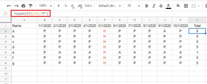
Here’s the formula I used in L2 to count presents, dragged down to L8:

=COUNTIF(B2:K2, "P")

Now, I don’t want to see columns B to K all the time. So I’ll group them.

Steps:

1. Select columns B to K
2. Right-click > View more column actions > Group columns B–K
3. Click the – button to collapse (hide), and + to expand (unhide)

Super handy!

Remove the Grouping

Right-click the line above the grouped columns (or on the + button), and choose “Remove group.”

What About Rows?

Same steps. Just select the rows instead of columns, group them, and you’ll see a similar +/- toggle on the left side.

This is perfect when you’re dealing with grouped data or want to make your sheet look cleaner without deleting anything.

Option 3 – Use Filters to Conditionally Hide Rows

This one’s different — and powerful. You can hide and unhide rows in Google Sheets based on the values in them using the filter feature.

Note: This only works for rows, not columns.

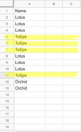
Example: Hide Rows Containing “Tulips”

Let’s say column A lists flower names, and you want to hide rows that say “Tulips.”

Here’s how:

1. Select A1:A13 (or the full column A if you want to include future data)
2. Go to Data > Create a filter
3. Click the little filter icon in cell A1
4. Uncheck Tulips and click OK

And just like that, rows with “Tulips” are hidden.

To unhide:

• Check “Tulips” again in the filter dropdown
• Or turn off the filter entirely (Data > Remove filter)

Which Method to Use for Hiding or Unhiding Rows or Columns

So there you go — three practical ways to hide and unhide rows or columns in Google Sheets:

• The usual way (quick and simple)
• Grouping (great for toggling repeated data)
• Filters (for conditional row hiding)

Pick the one that suits your situation best.

Resources

• How to Hide Formulas in Google Sheets
• How to Hide Tabs from Specific People in Google Sheets
• How to Group Rows and Columns in Google Sheets
• Grouping and Subtotal in Google Sheets and Excel
• Display Totals for Collapsed Groups and Subgroups in Google Sheets