As a webmaster, I often compare my current week’s traffic with the same week last year. While tools like Google Analytics can handle this, what if your data lives in Google Sheets? This tutorial will show you how to compare current and same week last year in Google Sheets using simple and dynamic formulas.

You might want to analyze performance metrics like site traffic, sales, or support volume over time. The key is to align complete weekly ranges to avoid skewed comparisons.

Note: In this guide, “current week” refers to the most recently completed full calendar week (Sunday to Saturday). This ensures a fair comparison between equivalent weeks across years.

Real-World Use Cases

Here are a few examples where comparing the current and same week last year in Google Sheets is helpful:

• Sales reporting: Track revenue patterns across seasons or promotions.
• Inventory management: Compare product movement by week to forecast demand.
• Support trends: See if ticket volume increased in the same week year-over-year.
• Website analytics: Understand long-term traffic performance and seasonality.

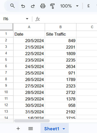
Sample Data

You’ll need a basic dataset with at least two columns:

• Column A: Dates
• Column B: Weekly metric (e.g., traffic, sales, etc.)

Filter Current and Same Week Last Year in Google Sheets

Current Week (Most Recent Full Sunday–Saturday Range)

Use the following formula to get the most recently completed full week:

=FILTER(A2:B, 
   ISBETWEEN(A2:A, 
      TODAY() - WEEKDAY(TODAY(), 1) - 6, 
      TODAY() - WEEKDAY(TODAY(), 1)
   )
)

Same Week Last Year

To fetch the same calendar week from the previous year:

=FILTER(A2:B, 
   ISBETWEEN(A2:A, 
      (TODAY() - WEEKDAY(TODAY(), 1) - 6) - 364, 
      (TODAY() - WEEKDAY(TODAY(), 1)) - 364
   )
)

Formula Explanation

Let’s break down the logic behind the formula used to compare current and same week last year in Google Sheets.

Part 1: TODAY()

Returns the current date. All calculations revolve around today.

Part 2: WEEKDAY(TODAY(), 1)

Returns a number from 1 (Sunday) to 7 (Saturday) that tells us what day of the week today falls on.

Part 3: TODAY() - WEEKDAY(TODAY(), 1)

Finds the last Saturday (end of the most recent full week).

Part 4: TODAY() - WEEKDAY(TODAY(), 1) - 6

Finds the previous Sunday (start of the most recent full week).

So,

ISBETWEEN(A2:A, start_of_week, end_of_week)

filters only the rows within that 7-day span.

Last Year’s Week Range

We subtract 364 days (52 weeks × 7) from both start and end of the current week, giving us the same week one year earlier:

(start_of_week - 364, end_of_week - 364)

This method ensures you’re comparing week-to-week properly, not just arbitrary dates.

Compare Totals with QUERY

To compare total values from both weeks:

Step 1: Stack the Two Weeks

=VSTACK(
   FILTER(A2:B, ISBETWEEN(A2:A, TODAY() - WEEKDAY(TODAY(), 1) - 6, TODAY() - WEEKDAY(TODAY(), 1))),
   FILTER(A2:B, ISBETWEEN(A2:A, (TODAY() - WEEKDAY(TODAY(), 1) - 6) - 364, (TODAY() - WEEKDAY(TODAY(), 1)) - 364))
)

Step 2: Group by Year Using QUERY

=QUERY(
   VSTACK(
      FILTER(A2:B, ISBETWEEN(A2:A, TODAY() - WEEKDAY(TODAY(), 1) - 6, TODAY() - WEEKDAY(TODAY(), 1))), 
      FILTER(A2:B, ISBETWEEN(A2:A, (TODAY() - WEEKDAY(TODAY(), 1) - 6)-364, (TODAY() - WEEKDAY(TODAY(), 1)-364)))
   ), "Select sum(Col2) pivot year(Col1)"
)

Output Example:

Use Monday–Sunday Weeks in Google Sheets (Optional)

By default, this tutorial uses a Sunday–Saturday week structure, which matches the behavior of WEEKDAY(..., 1) in Google Sheets. But if your reporting starts on Monday and ends on Sunday, you can easily adjust the formulas.

This is especially useful for businesses that follow a Monday-based workweek.

Modify the Formula for Monday–Sunday Weeks

To change the week start to Monday, use WEEKDAY(date, 2) instead of WEEKDAY(date, 1). This makes Monday = 1 and Sunday = 7.

Filter the Most Recent Full Week (Monday to Sunday)

=FILTER(A2:B, 
   ISBETWEEN(A2:A, 
      TODAY() - WEEKDAY(TODAY(), 2) - 6, 
      TODAY() - WEEKDAY(TODAY(), 2)
   )
)

Filter the Same Week Last Year

Just subtract 364 days (52 weeks) from both start and end:

=FILTER(A2:B, 
   ISBETWEEN(A2:A, 
      (TODAY() - WEEKDAY(TODAY(), 2) - 6) - 364, 
      (TODAY() - WEEKDAY(TODAY(), 2)) - 364
   )
)

Tip: This small tweak allows your comparison logic to align with international or corporate standards that treat Monday as the first day of the week.

Conclusion and Final Thoughts

And that’s how you can compare current and same week last year in Google Sheets using formulas. Whether you’re tracking traffic, sales, or other KPIs, this method gives you an accurate week-over-week comparison without relying on third-party tools.

Related Resources

• Compare Same Day Last Week Data in Google Sheets
• Finding Week Start and End Dates in Google Sheets
• Filter Data for a Specific Number of Past Weeks in Google Sheets
• Calculate Week Number Within Month (1–5) in Google Sheets
• Find the Date or Date Range from Week Number in Google Sheets
• How to Sum Values by the Current Week in Google Sheets
• Weekday Name to Weekday Number in Google Sheets
• Combine Week Start & End Dates with Calendar Week Formula
• Filter Data by Week (This, Last, or N Weeks Ago)
• How to Sum by Week of the Month in Google Sheets
• Convert Dates to Week Ranges in Google Sheets (Array Formula)