In order to use the current sheet name as the criterion in Google Sheets formulas, first, you must know how to get the current sheet name in a cell.
You can find Google Apps Script for that online. Here I am sharing with you a workaround that involves only the built-in Google Sheets functions.
The workaround will do the job nicely, but you should refresh the sheet(s) to get the change applied. The good part is that you can do that (the refreshing) by just tapping the DELETE button in a blank cell.
Introduction
I don’t know how many of you use the default sheet names in a Google Sheet file, that contains several sheets.
It’s quite common that we use meaningful names to rename the sheets. In such scenarios, if we want, we can use the sheet names as the criteria in formulas in Google Sheets.
The default sheet names in Google Sheets will be like “Sheet1”, “Sheet2”, “Sheet3”, “Sheet4”, and so on. Assume we have renamed these sheets to “Master”, “Apple”, “Mango”, “Orange” and so on.
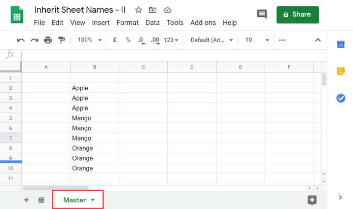
I have a list of fruit names in a column in the sheet titled “Master”.
What I want is to use a Filter formula in the sheet “Apple” that filters the fruits from the “Master” sheet by inheriting the sheet name “Apple” as the criterion.
When I use the same formula (without any modification) in the other two sheets, the formulas should filter the fruits based on the corresponding sheet names.
That means “Apple” filtered to the “Apple” tab, “Mango” filtered to the “Mango” tab, and “Orange” filtered to the “Orange” tab.
How can we do this without using an Apps Script in Google Sheets?
Using Current Sheet Name as the Criterion in Formulas in Google Sheets
Sample Data
Sample data is the essence of any formula test. So, first I will give you the sample data then the “things to do” to use the current sheet name as the criterion in formulas in Google Sheets.
Sample Data:

Things to Do (Workaround Requirements)
As I have told you at the very beginning of this tutorial, I am following a workaround approach to use the current sheet name as the criterion in Google Sheets.
For the workaround, we should keep the first-row blank in all the sheets. Further, we won’t use the “Master” sheet for data manipulation! Then?
What we will do is, we will copy the “Master” sheet, rename it, and then use it. Didn’t get? Please just read on.
Let’s see how to inherit the current sheet name dynamically in the first row in the “Master” sheet. So that we can later use the sheet names dynamically in formulas in other sheets.
There are three things to do.
1. In cell A1 in the “Master” sheet insert the below RAND formula.
=rand()We will use it to refresh the sheet later.
2. In cell B1 insert the below simple formula.
=Master!A1In this, “Master” is the sheet tab name. The formula simply returns the A1 value whatever it is.
3. Here is the third formula which is inserted in cell C1.
=REGEXEXTRACT(FORMULATEXT(B1),"[a-zA-Z ]+")In this, the FORMULATEXT returns the formula in B1 as a text. The REGEXEXTRACT is to extract the sheet name from the formula returned by the FORMULATEXT.
The result will be “Master” in cell C1 which is the sheet name of the current sheet.
We won’t use any data manipulation formula in this sheet. Then?
We will copy the sheet and change the copied sheet name as per the criteria requirement in data manipulation. I’ll come to that later.
You may now select row # 1 (in “Master”) and change the font color to white so that it will be hidden from views.
We are now fully set to use the current sheet name as the criterion in our formulas in Google Sheets.
Current Sheet Name as the Criterion in Filter Formula in Google Sheets
Here we are going to use the above sample sheet. Let’s understand the filter scenario first.
Assume I want to filter “Apple” from a list in the sheet named “Apple” and the criterion should be inherited from the sheet name itself. The criterion is “Apple” and here is how to do it.
Right-click on the sheet name “Master” and click “Duplicate”.
It’ll create a new sheet named “Copy of Master”. Double click on “Copy of Master” and type “Apple” to rename it.
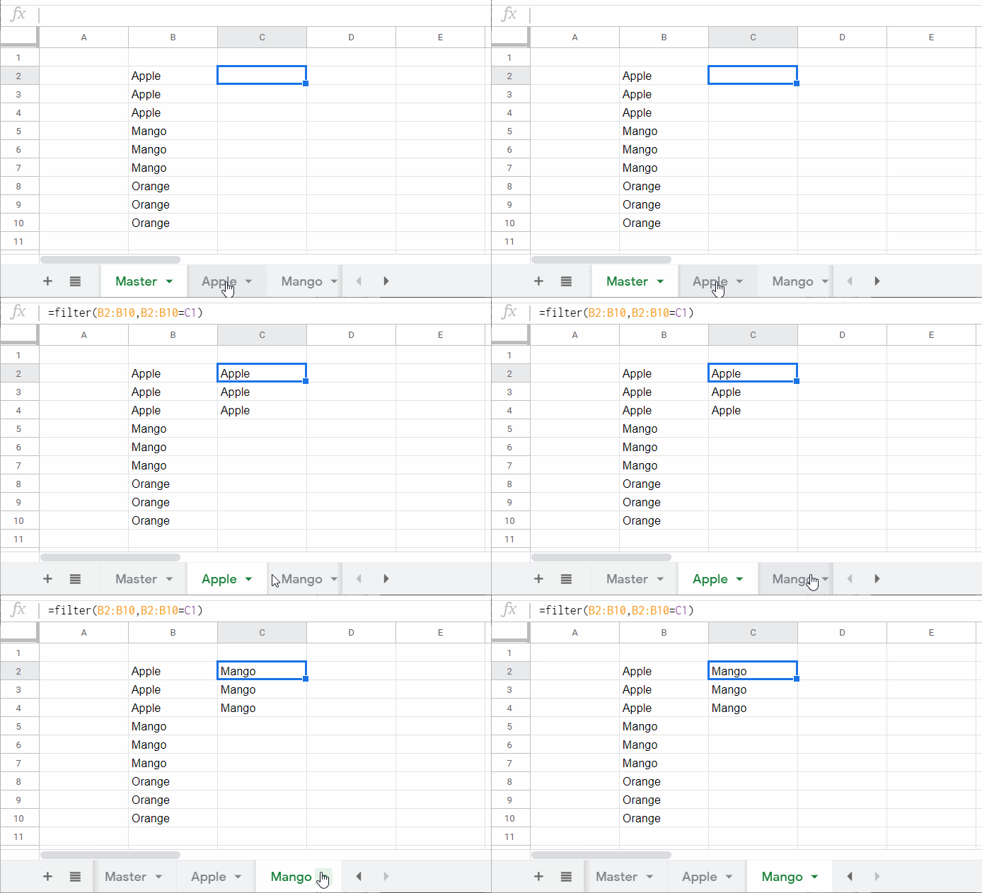
In this new sheet, insert the below formula in cell C2. It’s for filtering the values in B2:B10 for the values in B2:B10 match the criterion in C1 (current sheet name).
=filter(B2:B10,B2:B10=C1)The above FILTER formula would return #N/A! error. Let’s forget about it for the time being.
Now right-click on the sheet name “Apple” and select “Duplicate”. It will create a new sheet “Copy of Apple”. Change its name to “Mango”.
Now we have a total of three sheets – “Master”, “Apple”, and “Mango”. We have one filter formula each in cell C2 in the second and third sheets.
In any blank cell in any sheet, just tap the DELETE (delete) button on your keyboard. Check the results in “Apple” and “Mango” Sheets.
The Filter formula in the sheet “Apple” has used the criteria “Apple” to filter the fruit list. Similarly, the filter formula in the sheet “Mango” has used the criteria “Mango” to filter the fruit list!
The formulas successfully inherit the current sheet name as the condition. Cool, right?

Can we use the current sheet name as the criterion in the IMPORTRANGE function in Google Sheets?
Why not?
We can use the above method in functions that uses criterion from a cell. Here is one more example using QUERY with IMPORTRANGE.
Inherit Current Sheet Name and Use It in Query Importrange Formula
We use Query with Importrange to conditionally import data from one Google Sheets file to another Google Sheets file.
We can use our above method to import specific data dynamically to each tab in Google Sheets. Let’s see how.
Here are the two files – “Invoice – All in one” and “Invoice – Party Wise” that I am going to use in my following example.
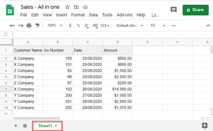
Sample Data (in Source File)
Here is the sample data in “Invoice – All in one”.

We are going to import part of the above data to each sheet in the file “Invoice – Party Wise”.
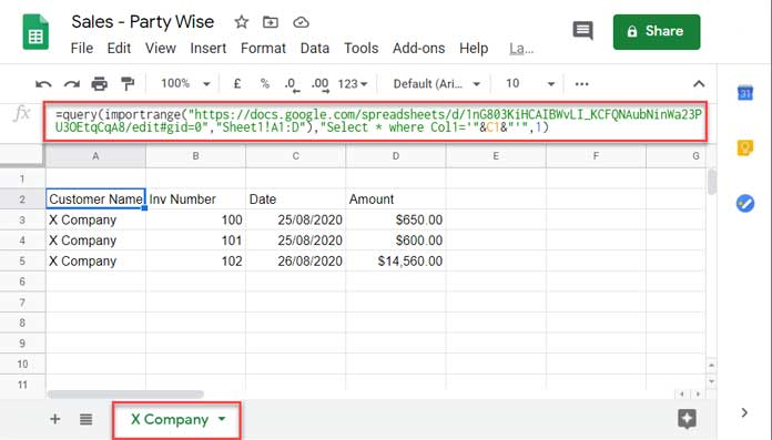
I mean, in “Invoice – Party Wise”, I have the following sheet which is named as “X Company”. In which I want to filter the data from “Invoice – All in one” that corresponds to “X Company”.
Destination File (Blank)
Open the blank file “Invoice – Party Wise” and rename the very first sheet as “X Company”.
Now let’s see how to import the data, query it as per the current sheet name as the criterion.
In cell A1 use the following RAND formula.
=rand()Then in cell B1 insert the formula ='X Company'!A1 (the apostrophe around the sheet name is mandatory if the sheet name contains a space character in between).
Now let’s insert the REGEXEXTRACT to extract the current sheet name in cell C1.
=REGEXEXTRACT(FORMULATEXT(B1),"[a-zA-Z ]+")Select the row#1 and change the font color to white as earlier.
We have completed the workaround to use the current sheet name as the criterion in our Query Importrange formula.
Importing Data into Destination File
To import the data, in cell A2, insert the following formula.
=importrange("URL_of_Sales-All_in_one_Here","Sheet1!A1:D")It will definitely return #REF! error.
Point your mouse over the error and click on “Allow Access”.
The formula will start importing all the data from the “Sales – All in one” file to the range A2:D11 in “Sales – Party Wise”.
The current sheet that contains the Importrange formula is “X Company”. So I just want to import the data specific to this company.
We can use Query with Importrange and use the current sheet name as the condition in the Query formula. How?
Current Sheet Name as the Criterion in Google Sheets Query
Wrap the Importrange formula with the Query as below.
=query(importrange("URL_of_Sales-All_in_one_Here","Sheet1!A1:D"),"Select * where Col1='"&C1&"'",1)
Duplicate this sheet tab and change the sheet name to “Y Company” and make one more duplicate and rename it to “Z Company”.
Tap the delete button in any blank cell. The Query Importrange formula will inherit the criteria from the sheet names itself.
That’s all. Enjoy!


