")
")


")


")

")
")
 in Excel & Google Sheets")


Merged cells often make spreadsheets look cleaner, but they break many formulas — especially COUNTIF and COUNTIFS. If you’re trying to count based on values in merged cells, you’ll likely get incorrect results… unless you know this workaround.
In this tutorial, I’ll show you how to correctly use COUNTIF and COUNTIFS in merged cells in Google Sheets without unmerging them, using a clever LOOKUP trick.
Why COUNTIF Fails with Merged Cells
Let’s say you merge cells A1:A10 and enter a date. Only A1 actually contains the value; the rest are blank. So a formula like:
=COUNTIF(A1:A10, "2024-08-15")will only count one cell, even if the entire merged range visually appears to contain the date. This behavior causes misleading counts in datasets that use merged cells for grouping.
The Fix: Use LOOKUP to Fill Merged Cell Values Virtually
We can virtually “fill down” merged values into each row using this formula:
=ARRAYFORMULA(LOOKUP(ROW(A3:A14), IF(LEN(A3:A14), ROW(A3:A14)), A3:A14))What it does:
ROW(A3:A14)creates a list of row numbers.IF(LEN(A3:A14), ROW(A3:A14))marks only non-empty cells.LOOKUP(...)fills down the last seen non-empty value — simulating an unmerged range.
This virtual range can then be safely used with COUNTIF.
Correct COUNTIF for Merged Cells
Scenario:
You have dates in merged cells in column A and want to count how many consignments were dispatched on a specific date (in F3).
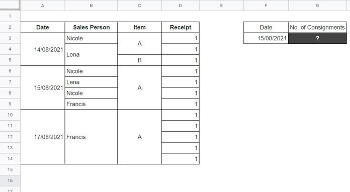
Incorrect (Standard) Formula:
=COUNTIF(A3:A14, F3)Correct Formula with LOOKUP:
=COUNTIF(
  ARRAYFORMULA(LOOKUP(ROW(A3:A14), IF(LEN(A3:A14), ROW(A3:A14)), A3:A14)),
  F3
)
This version accounts for merged cells and gives you the correct count.
Important: To get an accurate count, ensure there are no empty cells in the COUNTIF range—except for those created by merged cells. If it’s difficult to remove empty cells, consider entering a placeholder like “-” or “x” to exclude them from the count. You can do this easily by applying Data > Create a filter to the column and filtering for blanks. Also, use closed-ended ranges (e.g., A3:A14 instead of A3:A) to avoid counting unintended values outside your dataset.
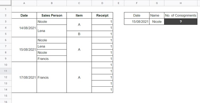
Using COUNTIFS with Merged Cells (Multiple Conditions)
Now let’s say you also want to count only if the person’s name in column B matches a specific value in G3.
Correct Formula with Multiple LOOKUPs:
=COUNTIFS(
  ARRAYFORMULA(LOOKUP(ROW(A3:A14), IF(LEN(A3:A14), ROW(A3:A14)), A3:A14)),
  F3,
  ARRAYFORMULA(LOOKUP(ROW(B3:B14), IF(LEN(B3:B14), ROW(B3:B14)), B3:B14)),
  G3
)
Example Output:
If F3 = 2021-08-15 and G3 = "Nicole", the formula will correctly return the number of consignments she dispatched on that date — even though the original data contains merged cells.
Bonus Tip: Hardcoding Criteria
Instead of using cell references like F3 and G3, you can hardcode the criteria:
=COUNTIFS(
  ARRAYFORMULA(LOOKUP(ROW(A3:A14), IF(LEN(A3:A14), ROW(A3:A14)), A3:A14)),
  DATE(2021, 8, 15),
  ARRAYFORMULA(LOOKUP(ROW(B3:B14), IF(LEN(B3:B14), ROW(B3:B14)), B3:B14)),
  "Nicole"
)
Summary: How to Handle Merged Cells with COUNTIF(S)
| Problem | Solution |
| COUNTIF/COUNTIFS fail on merged ranges | Use LOOKUP to simulate unmerged values |
| Need to count based on a merged column | Wrap the column in ARRAYFORMULA(LOOKUP(…)) |
| Using multiple criteria | Apply the LOOKUP trick to all criteria ranges |
Related Guides
- How to Count Merged Cells in Google Sheets (and Get Their Size) — A formula-based method that avoids counting extra empty cells below merged blocks, which is a common issue when using
COUNTIF. - How to Use SUMIF in Merged Cells in Google Sheets
- Copy and Paste Merged Cells Without Blank Rows in Google Sheets
- Uncover Merged Cell Addresses in Google Sheets
- Automatically Fill Merged Cells in Google Sheets – Down or Across
- Use SUMPRODUCT with Merged Cells
- How to Sort Vertically Merged Cells in Google Sheets
Thanks, it worked perfectly.