Empty cells in a row can carry significant meaning—for example, a missing sales or purchase entry in a sales report, or employee absences in an attendance sheet. You can use the COUNTBLANK function to count blank cells in rows in Google Sheets.
If you want to apply this function row by row, you must use it with the BYROW function. Before BYROW and LAMBDA were available, we had to rely on workarounds using functions like DSUM and MMULT.
However, the COUNTBLANK function won’t automatically apply row by row when used as an array formula. This is because COUNTBLANK itself is an array function—it returns the number of empty cells in a given range, but only as a single value.
Sample Data
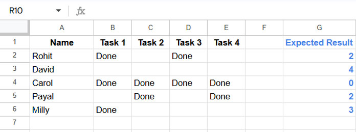
The following sample table contains employee names and their task statuses. We’ll count how many tasks are pending (i.e., how many blank cells) for each employee:

COUNTBLANK to Count Blank Cells in Rows in Google Sheets
The easiest way to count blank cells in each row is to use the COUNTBLANK formula in cell F2 and drag it down:
=COUNTBLANK(B2:E2)This returns the count of blank cells in each respective row.
Array Formula to Count Blank Cells Row by Row
If you prefer not to use a drag-down formula and want a more dynamic solution, you can use a custom LAMBDA function combined with BYROW:
=BYROW(B2:E6, LAMBDA(row_, COUNTBLANK(row_)))Here’s how it works:
LAMBDA(row_, COUNTBLANK(row_))defines a custom function that counts blank cells in a row.BYROWapplies that function to each row in the rangeB2:E6.
Why Use This Approach?
The LAMBDA and BYROW functions allow you to count blank cells in each row dynamically—ideal for datasets that update or expand frequently.
LAMBDA works by default in Google Sheets, but older alternatives like DSUM and MMULT are still useful for educational or compatibility reasons.
Count Blank Cells in Each Row Using DSUM
Before BYROW, one workaround was using the DSUM function. Though typically used for summing database fields, you can adapt DSUM to count blank cells in each row.
Here’s how:
- Convert blank cells to
1and non-blank cells to0. - Sum those values using DSUM after transposing the data.
Formula:
=ArrayFormula(
   DSUM(
      TRANSPOSE(HSTACK(B2:B6, --ISBLANK(B2:E6))),
      SEQUENCE(ROWS(B2:B6)),
      {IF(,,); IF(,,)}
   )
)Explanation:
--ISBLANK(B2:E6)converts TRUE/FALSE to 1/0 for blank/non-blank cells.HSTACK(B2:B6, …)adds the row labels required forDSUM.TRANSPOSEchanges the data orientation.SEQUENCE(ROWS(B2:B6))defines the fields.- The criteria
{IF(,,); IF(,,)}is a blank condition used to evaluate all rows.
This technique effectively counts blank cells in each row using database logic.
Count Blank Cells in Each Row Using MMULT
Another effective method is using matrix multiplication via MMULT:
=ArrayFormula(
   MMULT(
      --ISBLANK(B2:E6),
      TRANSPOSE(COLUMN(B2:E2)^0)
   )
)Explanation:
--ISBLANK(B2:E6)returns a 2D array with 1 for blank cells and 0 for filled ones.COLUMN(B2:E2)^0returns a horizontal array of1s matching the number of columns.TRANSPOSEconverts it into a vertical array, allowing matrix multiplication.
The result is a vertical array showing the count of blank cells for each row.
Resources
- Fill Blank Cells with the Next Non-Empty Value in Google Sheets
- Fill Blank Cells with Values from the Cell Above in Google Sheets
- Fill Empty Cells with the Value from Above in Excel
- How to Fill Empty Cells with 0 in Pivot Table in Google Sheets
- Count From First Non-Blank Cell to Last Non-Blank Cell in a Row in Google Sheets
- How to Sort Rows to Bring Blank Cells to the Top in Google Sheets


