Consolidate Only the Last Row in Multiple Sheets in Google Sheets

Data consolidation means combining values from multiple ranges in the same worksheet, multiple worksheets or multiple workbooks into one new range. Even though this post is about how to consolidate only the last row in multiple Sheets, it’s better to have a clear picture of the data consolidation first.

We normally use Query for consolidating data in Google Sheets. In Excel, there is a data consolidation command under the Data menu which is quite useful for newbies.

One thing is important in data consolidation is the structure of data. The data must be identical in the sheets. I mean the same number of columns, same data types in each column and must share common column names. But there is no restriction in the number of rows.

I have an elaborated tutorial on Google Sheets Data Consolidation. Still, here I am going to give you an overview of data consolidation. After that, we can go to how to consolidate the last row in multiple Sheets in Google Sheets.

Formula, Sample Data in Two Sheets and the Output:

=query({Sheet1!A1:D4;Sheet2!A2:D4},"Select Col1, sum(Col2),max(Col3),sum(Col4) group by Col1",1)
A quick overview of consolidating data

See how I have consolidated “sheet1” and “sheet2” in “sheet3”. I have summed column 2 (Qty) and column 4 (Amt). But as it’s visible I have used the Max Query scalar function.

This is because I don’t want to sum the rate. Since there is no way to return the rate without summing, the only way is to use the Max or Min to return the rate as it is. A cool tip, right?

How to Consolidate the Data in the Last Row in Multiple Sheets

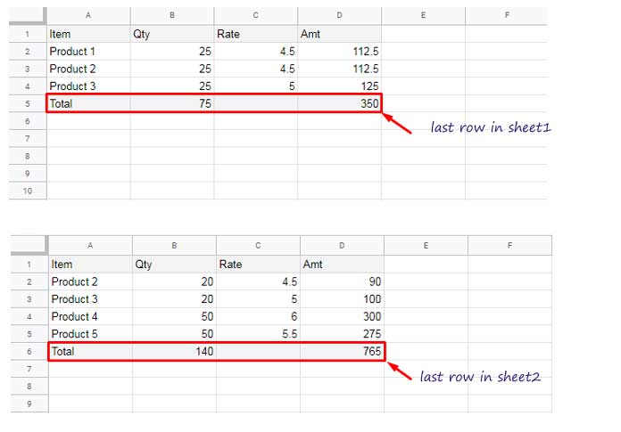
If you have a total row, the last row, containing the total of a column or columns in multiple identical Sheets, then you may want to consolidate them.

Here the only obstacle in front of you will be finding the last row in each sheet dynamically. I have the correct formula for that – Address of the Last Non-Empty Cell Ignoring Blanks in a Column in Excel. It works equally well in Docs Sheets.

I am going to use that to consolidate only the last row in multiple Sheets in Docs Sheets.

Sample data and last row marked

To consolidate only the last row in multiple Sheets, please follow the below step by step instructions.

Step 1:

Finding the Last Row Number to Offset

Sheet 1 Formula:

=ArrayFormula(MATCH(2,1/(Sheet1!A:A<>""),1))

Sheet 2 Formula:

=ArrayFormula(MATCH(2,1/(Sheet2!A:A<>""),1))

Enter the above formulas in “sheet3” in which I am going to consolidate the last row in “sheet1” and “sheet2”. The first formula would return 5 and the second would return 6.

Step 2:

Extracting the Last Row Using Index by Row Offset

We can use the Index function with the above formulas to offset 5 and 6 rows in each sheet and return the total (last) row. When using Index, you can omit the function ArrayFormula which I have used with the above two formulas.

Syntax:

INDEX(reference, [row], [column])

In this, we have already got the ‘row’ offset. Simply put 0 as ‘column’ offset to return the entire last row content.

Formula 1 to extract the last row in “sheet1”.

=index(Sheet1!A1:D,MATCH(2,1/(Sheet1!A:A<>""),1),0)

Formula 2 to extract the last row in “sheet2”.

=index(Sheet2!A1:D,MATCH(2,1/(Sheet2!A:A<>""),1),0)

Step 3:

Formula to Combine Last Rows of Multiple Sheets

Now you can combine the above two last rows prior to consolidating. I have included the title row too in the combining.

={Sheet1!A1:D1;index(Sheet1!A1:D,MATCH(2,1/(Sheet1!A:A<>""),1),0);index(Sheet2!A1:D,MATCH(2,1/(Sheet2!A:A<>""),1),0)}
Combine the last row in multiple Sheets

Step 4:

Google Sheets Formula to Consolidate Only the Last Row of Multiple Sheets

Just use the above formula in Query as data and summarize as below.

Consolidating the last row in multiple Sheets
=query({Sheet1!A1:D1;index(Sheet1!A1:D,MATCH(2,1/(Sheet1!A:A<>""),1),0);index(Sheet2!A1:D,MATCH(2,1/(Sheet2!A:A<>""),1),0)},"Select Col1,Sum(Col2),max(Col3),Sum(Col4) group by Col1",1)

You can include more than two sheets in this type of last row consolidation.

Any doubt adding more sheets or any other part of this tutorial, please do ask in the comments. Thanks for the stay. Enjoy!

Prashanth KV
Prashanth KV
Your Trusted Google Sheets and Excel Guide Prashanth KV brings a wealth of experience in Google Sheets and Excel, cultivated through years of work with multinational corporations in Mumbai and Dubai. As a recognized Google Product Expert in Docs Editors, Prashanth shares his expertise through insightful blogging since 2012. Explore his blog for practical tips and guidance on maximizing your spreadsheet skills.

Marking Case-Sensitive Unique Values in Excel

Marking case-sensitive unique values provides several benefits compared to merely extracting them in an...

Highlight Upcoming Birthdays in Google Sheets

When highlighting upcoming birthdays in Google Sheets, one important aspect is ignoring the year...

Compare Two Tables for Differences in Excel

To compare two tables with similar data for differences, you can use the XLOOKUP...

Calculate Weighted Average in Pivot Table in Google Sheets

You can calculate a weighted average in a Pivot Table using a custom formula...

More like this

Highlight Upcoming Birthdays in Google Sheets

When highlighting upcoming birthdays in Google Sheets, one important aspect is ignoring the year...

Calculate Weighted Average in Pivot Table in Google Sheets

You can calculate a weighted average in a Pivot Table using a custom formula...

Summarize Data and Keep the Last Record in Google Sheets

In Google Sheets, we can summarize data (like sum, average, min, max, count) using...

LEAVE A REPLY

Please enter your comment!
Please enter your name here

This site uses Akismet to reduce spam. Learn how your comment data is processed.