There is no LARGEIF function in Google Sheets. However, you can achieve conditional Large in Google Sheets by using the IF or FILTER function with LARGE.

You can include single or multiple conditions in LARGE using the IF or FILTER functions.

Regular Use of LARGE

See how the LARGE function works without any criteria or conditions.

Sample Data:

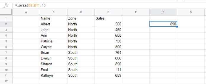
Large without Any Criteria in Google Sheets

The following formula returns the largest value (max value) in the selected range:

=LARGE(D2:D, 1)  // returns 890

To return the 3rd largest value, use the following formula:

=LARGE(D2:D, 3)  // returns 764

Now, let’s apply conditional LARGE, also known as LARGE IF in Google Sheets.

Single-Criteria LARGE Function in Google Sheets

Using IF Logical Test with LARGE

This is a LARGE + IF combination, serving as an equivalent to the non-existent LARGEIF function.

Suppose we want to find the highest sales volume in the “North” zone. We can use the following formula:

=ArrayFormula(LARGE(IF(C2:C="North", D2:D), 1))

Result: 800

The ArrayFormula is necessary because IF is not an array function, and we are referencing a range in it. The ArrayFormula enables IF to handle an array.

Using FILTER with LARGE

Here’s another formula to find conditional Large in Google Sheets using LARGE and FILTER:

=LARGE(FILTER(D2:D, C2:C="North"), 1)

This formula first filters the sales volume for the “North” zone and then applies the LARGE function.

Multi-Criteria LARGE Function in Google Sheets

Using IF Logical Test with Multiple Conditions in LARGE

Since we are using multiple criteria, the IF function requires an ArrayFormula. If you want to learn more about this, check out the tutorial How to Use IF, AND, OR in Array in Google Sheets.

Here’s a multiple-criteria LARGE formula that considers sales from “North” and “South” zones:

=ArrayFormula(LARGE(IF((C2:C="North")+(C2:C="South"), D2:D), 1))

The above formula returns the highest sales volume from both “North” and “South” zones.

To add one more condition (e.g., “East”), modify the formula as follows:

=ArrayFormula(LARGE(IF((C2:C="North")+(C2:C="South")+(C2:C="East"), D2:D),1))

However, for multiple criteria in LARGE, I recommend using the LARGE + FILTER + XMATCH combination for better readability and efficiency.

Using FILTER and XMATCH Combo with LARGE

Here are two examples demonstrating conditional Large in Google Sheets using LARGE, FILTER, and XMATCH:

Largest sales volume from North and South regions:

=LARGE(FILTER(D2:D, XMATCH(C2:C, {"North", "South"})), 1)

Largest sales volume from North, South, and East regions:

=LARGE(FILTER(D2:D, XMATCH(C2:C, {"North", "South", "East"})), 1)

In these formulas, XMATCH returns either a number (if the condition is met) or an #N/A error (if it isn’t). The FILTER function then filters the rows that match the condition.

Conclusion

That’s all about conditional Large in Google Sheets! By leveraging LARGE, IF, FILTER, and XMATCH, you can efficiently find the highest values based on conditions.

Additional Resources

• Find Top N Values with Criteria in Google Sheets (MAX/LARGE) – With Tie-Breaking
• Find the Largest Date in Each Group in Google Sheets
• Find and Filter the Min or Max Value in Groups in Google Sheets