Before applying conditional indentation in Google Sheets, it’s important to understand what it is.

In document writing, indentation is the space added at the beginning of a line, typically to mark the start of a paragraph. In spreadsheets, indentation can be used to format text hierarchically.

Conditional indentation dynamically adjusts the number of spaces before text based on values in another column. This allows you to visually represent different hierarchy levels within a text column.

Example

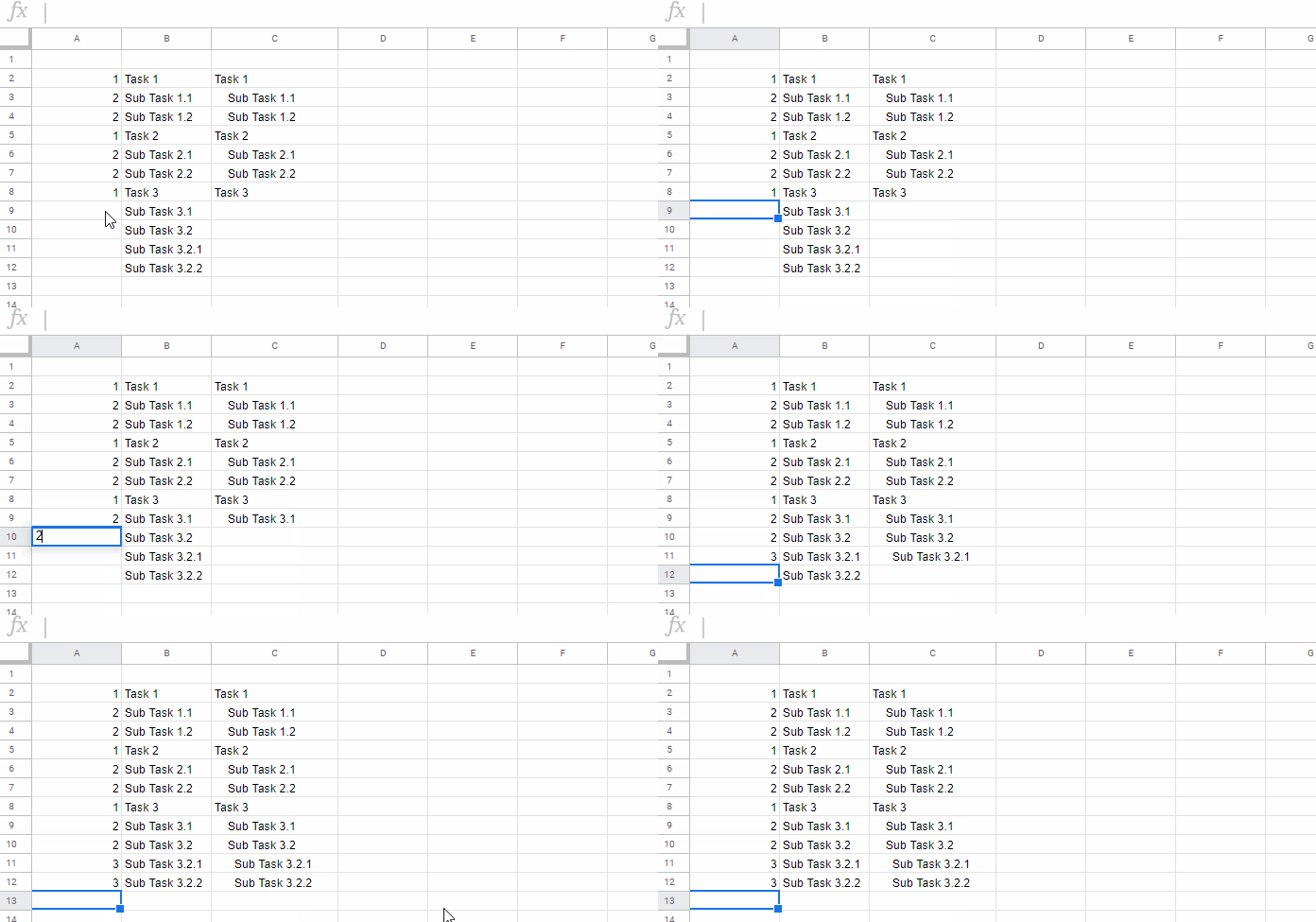
In this example, the array formula in cell C2 uses the conditions in A2:A to determine how much indentation to apply to the text in B2:B. The result appears in C2:C. Once applied, you can hide columns A and B to display only the indented text.

Five-Tier Conditional Indentation Formula in Google Sheets

In the above example, we used a five-tier indentation formula in cell C2. This means it accepts the numbers 1 to 5 in column A to apply indentation accordingly.

Let’s first understand the sample data in column B and the corresponding numbers in column A.

Conditional Indentation Example in Google Sheets

• The numbers in column A determine the indentation level.
• The corresponding values in column B are indented based on these numbers.
• “Task 1,” “Task 2,” and “Task 3” in column B are top-level tasks that should not be indented, so they are assigned a value of 1 in column A.
• When the number increases in column A, the formula increases the indent accordingly.

This demonstrates how conditional indentation in Google Sheets allows dynamic formatting based on predefined conditions.

Applying the Conditional Indentation Formula

Use the following five-tier conditional indentation formula in cell C2, covering the range A2:B:

=ArrayFormula(
   IF(LEN(A2:A), 
      SWITCH(A2:A, 
         2, TEXT(B2:B, REPT(" ", 2)&"@"), 
         3, TEXT(B2:B, REPT(" ", 6)&"@"), 
         4, TEXT(B2:B, REPT(" ", 10)&"@"), 
         5, TEXT(B2:B, REPT(" ", 14)&"@"), 
         B2:B
      ), ""
   )
)

Expanding the Indentation Levels

To add another level of indentation, insert this line before B2:B in the formula:

6, TEXT(B2:B, REPT(" ", 18)&"@"),

Formula Explanation

This formula consists of two main parts:

1. IF + LEN Check: Ensures the formula only applies when there are values in column A.
2. SWITCH Function: Determines the indentation level based on the values in column A.

Here’s the general structure of the formula:

=ArrayFormula(IF(LEN(A2:A), switch_formula, ""))

This means that if there are values in A2:A, the SWITCH formula executes; otherwise, the cell remains blank.

Breakdown of the SWITCH Formula

SWITCH(A2:A, 
         2, TEXT(B2:B, REPT(" ", 2)&"@"), 
         3, TEXT(B2:B, REPT(" ", 6)&"@"), 
         4, TEXT(B2:B, REPT(" ", 10)&"@"), 
         5, TEXT(B2:B, REPT(" ", 14)&"@"), 
         B2:B
)

In simple terms:

• If A2:A = 2, insert 2 spaces.
• If A2:A = 3, insert 6 spaces.
• If A2:A = 4, insert 10 spaces.
• If A2:A = 5, insert 14 spaces.
• Otherwise, return the original text in B2:B.

Each indentation level increases by 4 spaces to create a visually structured list.

Understanding SWITCH Syntax

SWITCH(expression, case1, value1, [case2, value2, …], [default_value])

• The expression here is A2:A.
• The numbers 2, 3, 4, and 5 are the cases.
• The corresponding TEXT formulas are the values returned.
• If no case matches, the default value (B2:B) is used.

Conclusion

This approach to conditional indentation in Google Sheets allows you to format text dynamically based on predefined conditions, making structured data easier to read.

Related Resources

• Inserting Bullet Points in Google Sheets
• Increase and Decrease Indent in Google Sheets with Macro
• 5-Star Rating in Google Sheets Including Half Stars
• Rate with Ease: Google Sheets’ New Built-In Rating Feature
• Insert Special Characters Without an Add-on in Google Sheets
• Clean Function in Google Sheets and Non-Printable Characters
• How to Create First Line Indent and Hanging Indent in Google Docs