Concatenating columns in Google Sheets can sometimes save a lot of time. For example, you may have first and last names in separate columns. Instead of manually combining them, you can use a formula to merge them into a single column.

In other cases, concatenation can simplify data entry. For example, if you have product codes as sequences in one column and product text IDs in another, you can generate a sequence using the SEQUENCE function in one column and enter product text IDs in another column before combining them.

To concatenate multiple columns in a row, you can use functions such as CONCATENATE, JOIN, TEXTJOIN, and the & (Ampersand) operator. When working with multiple-column ranges, you should use ARRAYFORMULA or the BYROW/MAP lambda functions.

Concatenate Multiple Columns in a Row

Consider the following dataset:

The range A2:E2 represents the data without headers. Let’s concatenate these columns in F2.

Using Ampersand

=A2&" "&B2&", "&C2&", "&D2&", "&E2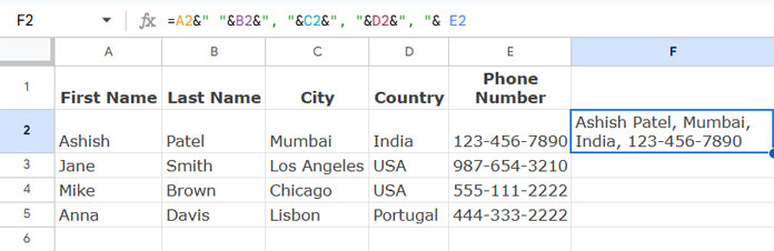

This formula:

• Adds a space between the first and last name.
• Separates address components with a comma followed by a space.

Note:

• You must specify each cell and delimiter individually.
• It allows flexibility in choosing delimiters.
• It removes number or date formatting. Use TEXT to retain formatting.

Example: If B2 contains a date, use:

TEXT(B2, "DD/MM/YYYY")

If B2 contains currency, use:

TEXT(B2, "$##.00")

Using CONCATENATE

This function works similarly to the Ampersand approach:

=CONCATENATE(A2, " ", B2, ", ", C2, ", ", D2, ", ", E2)

Key Points:

• Requires specifying each cell and delimiter manually.
• Allows flexibility in choosing delimiters.
• Removes number and date formatting (use TEXT to preserve them).

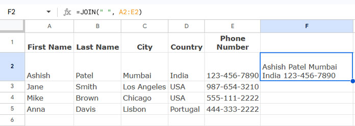
Using JOIN

=JOIN(" ", A2:E2)

Advantages:

• Allows specifying a delimiter while concatenating a range.
• Retains number and date formatting.

Limitations:

• Cannot use different delimiters between columns.

This formula produces:

Using TEXTJOIN

=TEXTJOIN(" ", TRUE, A2:E2)

Benefits:

• Works like JOIN, but allows excluding empty cells.
• The TRUE argument ensures empty cells are skipped.
• Retains number and date formatting.

If you want to include empty cells, change TRUE to FALSE.

Concatenate Multiple Columns in Each Row

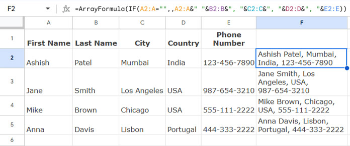
Now, let’s concatenate multiple columns for multiple rows. Suppose you have addresses of several people in the range A2:E. You can apply formulas to all rows instead of dragging down manually.

Using Ampersand with ARRAYFORMULA

=ArrayFormula(IF(A2:A="",,A2:A&" "&B2:B&", "&C2:C&", "&D2:D&", "&E2:E))

• Expands the formula to multiple rows.
• Returns a blank if the first column (A2:A) is empty.

Using CONCATENATE with MAP

Using CONCATENATE for multiple rows requires MAP:

=MAP(
   A2:A, B2:B, C2:C, D2:D, E2:E, 
   LAMBDA(col_1, col_2, col_3, col_4, col_5, IF(col_1="",, 
      CONCATENATE(col_1, " ", col_2, ", ", col_3, ", ", col_4, ", ", col_5)
   ))
)

Here’s how it works:

• MAP processes each row individually.
• LAMBDA assigns variable names (col_1, col_2, etc.) for use inside CONCATENATE.

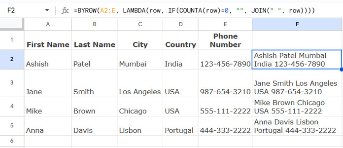
Using JOIN with BYROW

=BYROW(A2:E, LAMBDA(row, IF(COUNTA(row)=0, "", JOIN(" ", row))))

• BYROW applies JOIN row-wise.
• This method is useful when concatenating a large number of columns.

Using TEXTJOIN with BYROW

=BYROW(A2:E, LAMBDA(row, TEXTJOIN(" ", TRUE, row)))

• More efficient than JOIN.
• Can exclude empty cells automatically.

Handling Large Datasets

Concatenation may break if applied to several hundred rows. Functions like MAP and BYROW use lambda functions, which can slow down performance.

For large datasets, consider using QUERY as an alternative:

=TRANSPOSE(QUERY(TRANSPOSE(A2:E),,9^9))

• This approach efficiently concatenates all columns in each row.
• It does not allow custom delimiters (defaults to a space).

Summary

To concatenate columns in Google Sheets efficiently:

• Use & or CONCATENATE for flexibility.
• Use JOIN or TEXTJOIN for simplicity.
• Use ARRAYFORMULA or BYROW for multi-row concatenation.
• Use QUERY for large datasets.

Additional Resources

• How to Properly Concatenate Start Time with End Time in Google Sheets
• Concatenate Header Names with Cell Values in Google Sheets
• Concatenating Double Quotes with Text in Google Sheets
• Concatenate a Number Without Losing Its Format in Google Sheets
• Query to Combine Columns and Add Separators in Google Sheets
• A Flexible Array Formula for Joining Columns in Google Sheets