When handling data in Google Sheets, it’s common to ask: does a row contain any of the values I’m looking for? Manually scanning through rows can be time-consuming, especially if your dataset is large.

For example, imagine you have a list of names spread across several columns, and you need to check if Ann, Steven, or Clara appears in each row. Instead of searching cell by cell, you can set up a formula that automatically returns TRUE if at least one of those names is present in the row—or FALSE if none of them are found.

This approach is useful in many scenarios, such as:

• Checking attendance records to see if certain students are listed.
• Verifying whether product codes or IDs appear in a row of inventory data.
• Searching for specific keywords in text-based datasets.

In this tutorial, I’ll show you how to check row-wise if any of the values are present in columns using simple Google Sheets formulas, so you can save time and reduce errors.

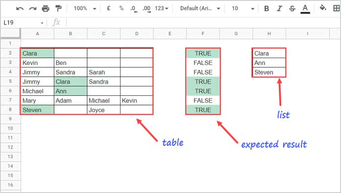
Sample Data and Expected Output

In this example, the sample data is in A2:D, and the list of values to search for is in H2:H4.

The expected output is in F2:F:

Formula to Check If a Row Contains Specific Values in Google Sheets

In cell F2, enter the following formula and drag it down as far as you need:

=SUMPRODUCT(IFNA(XMATCH(A2:D2, $H$2:$H$4)))>0

How the Formula Works

• XMATCH – Checks whether the values in A2:D2 exist in the list H2:H4 and returns their relative positions. If not found, it returns #N/A.
• IFNA – Replaces #N/A with blank results.
• SUMPRODUCT – Calculates the sum of matches.
• If the result is greater than 0, the formula outputs TRUE, meaning at least one of the specified values is present in the row. Otherwise, it returns FALSE.

This is the simplest way to check if a row contains specific values in Google Sheets.

Array Formula Version with BYROW

If you’d rather spill the results automatically (instead of dragging down the formula), you can use BYROW with a custom LAMBDA function:

=BYROW(A2:D, LAMBDA(row, SUMPRODUCT(IFNA(XMATCH(row, H2:H4)))>0))

This version applies the same logic row by row and spills results for the entire range.

Use Cases of Checking Row-Wise Values in Google Sheets

Here are some practical scenarios where this method can save time:

• Attendance tracking – Quickly verify if certain students are marked present in a row.
• Inventory management – Check whether specific product IDs or SKUs appear in stock records.
• Survey responses – Identify if any target keywords are mentioned in multi-column response data.
• Data cleaning – Detect rows that contain required values before filtering or processing.
• Project tracking – Confirm whether assigned team members are listed across task rows.

Resources

If you found this tutorial helpful, here are more guides on searching and matching data in Google Sheets:

• Search Across Columns and Return the Header in Google Sheets
• Create a Multi-Column Search Box in Google Sheets
• HLOOKUP to Search Entire Table and Find the Header in Google Sheets
• Multiple Search Strings in a SEARCH Formula for Google Sheets
• VLOOKUP to Search Across Multiple Columns in Google Sheets
• How to Search Across Multiple Columns with XLOOKUP in Google Sheets