


")


")

")
")
 in Excel & Google Sheets")


The standard VLOOKUP function in Google Sheets is case-insensitive. However, you can perform a case-sensitive VLOOKUP in Google Sheets by combining it with helper functions like EXACT, REGEXMATCH, or CODE.
This tutorial walks you through simple, practical methods to implement case-sensitive lookups with easy-to-follow examples.
Comparison Table: Methods for Case-Sensitive VLOOKUP
| Method | Description | Use Case |
|---|---|---|
| EXACT + VLOOKUP | Uses EXACT for strict case comparison | Recommended for simple, clean implementation |
| REGEXMATCH + VLOOKUP | Uses regex to match case-sensitive patterns | Good for partial/word-boundary matching |
| CODE + VLOOKUP | Compares character codes | More complex; rarely preferred |
| XLOOKUP / FILTER / INDEX-MATCH | Alternatives to VLOOKUP supporting case sensitivity | More flexible and readable |
Sample Data and Case-Insensitive VLOOKUP Formula
In column A, we have product IDs, column B contains corresponding descriptions, and column C shows the available quantities. We’ll use this table to demonstrate a case-sensitive VLOOKUP.
Some product IDs differ only by case. For example, SH_101A and SH_101a both refer to safety helmets from different makes.
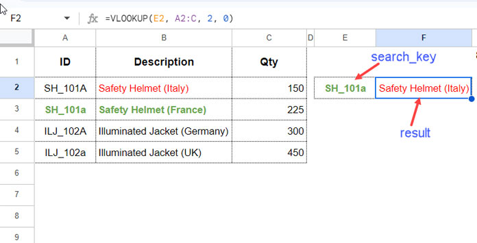
Let’s say you want to look up a product name based on an ID entered in cell E2:
=VLOOKUP(E2, A2:C, 2, 0)This standard formula returns the second column value that matches the search key in column A. However, since VLOOKUP is case-insensitive, it may return incorrect results when dealing with IDs that differ only in case.
To fix that, let’s explore how to use a case-sensitive VLOOKUP in Google Sheets using EXACT, REGEXMATCH, and CODE.
Case Sensitive VLOOKUP Using EXACT
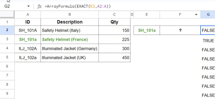
The EXACT function checks whether two strings match exactly, including letter casing.
Here’s how you can use it with ArrayFormula:
=ArrayFormula(EXACT(E2, A2:A))This returns an array of TRUE or FALSE values, depending on whether each cell in column A exactly matches E2.
Use with VLOOKUP
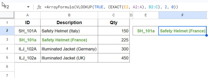
You can feed this result into a virtual range using HSTACK or curly braces:
=ArrayFormula(VLOOKUP(TRUE, {EXACT(E2, A2:A), B2:C}, 2, 0))Here, TRUE is used as the lookup value because the first column of the virtual range is now a series of TRUE/FALSE values.
Spill Formula (Multiple Search Keys)
If you have multiple search keys (for example, in E2:E4), use this MAP version:
=MAP(E2:E4, LAMBDA(r, ArrayFormula(VLOOKUP(TRUE, {EXACT(r, A2:A), B2:C}, 2, 0))))Tip: If you’re manually copying the non-spill formula down (instead of using the MAP version), make sure to convert the ranges to absolute references — for example, change A2:A to $A$2:$A and B2:C to $B$2:$C.
Case Sensitive VLOOKUP Using REGEXMATCH
This is a similar approach using REGEXMATCH. Instead of EXACT, use:
REGEXMATCH(A2:A, "^" & E2 & "$")This checks for an exact full-string match, respecting case.
Case-Sensitive Formula with REGEXMATCH
=ArrayFormula(VLOOKUP(TRUE, {REGEXMATCH(A2:A, "^"&E2&"$"), B2:C}, 2, 0))Partial Match (Optional)
Want to allow partial whole-word matches? Replace the pattern with:
"\b" & E2 & "\b"This lets “ILJ_102A Wh#2” match “ILJ_102A”.
Spill Formula for Multiple Matches
=MAP(E2:E4, LAMBDA(r, ArrayFormula(VLOOKUP(TRUE, {REGEXMATCH(A2:A, "^"&r&"$"), B2:C}, 2, 0))))Case Sensitive VLOOKUP Using CODE
This method is less flexible but helpful to understand, especially when reviewing shared sheets.
Since CODE only returns the Unicode value of the first character, we use MID and SEQUENCE to convert each character and concatenate the results.
Step 1: Add a Helper Column
In cell D2, enter:
=ArrayFormula(JOIN("", CODE(MID(A2, SEQUENCE(LEN(A2)), 1))))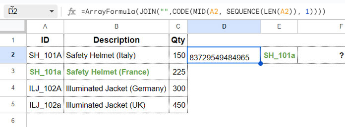
Drag it down as needed.
Step 2: VLOOKUP with CODE
Now convert the search key directly within the following formula (no helper column needed for it):
=VLOOKUP(ArrayFormula(JOIN("", CODE(MID(E2, SEQUENCE(LEN(E2)), 1)))), {D2:D, B2:C}, 2, 0)Because of the complexity and helper column requirement, I don’t recommend this method for most use cases.
Alternatives to Case Sensitive VLOOKUP in Google Sheets
If you prefer not to use VLOOKUP, these formulas also support case-sensitive lookups in Google Sheets:
XLOOKUP:
=ArrayFormula(XLOOKUP(TRUE, EXACT(E2, A2:A), B2:B))FILTER:
=FILTER(B2:B, EXACT(E2, A2:A))INDEX + MATCH:
=INDEX(B2:B, MATCH(TRUE, EXACT(E2, A2:A), 0))These methods offer flexible, readable, and often more efficient alternatives to case-sensitive VLOOKUP formulas.