Calculate Day Wise Working Hours in Google Sheets

This is an ultimate Spreadsheet tutorial that you can follow to calculate day wise working hours in Google Sheets.

No matter your employees are working in daytime, day and night, weekends, overtime, all you can calculate just from the work start and work end time.

In concise with the terms day wise working hours, I intend to say one thing. Split the working hours’ date wise.

If you are handling payroll and timekeeping of your employees, you can save your precious time by following this tutorial and also the sample sheet provided herewith.

You just need to enter the work start time, work end time and hourly rate for normal as well overtime hours. The corresponding cells are highlighted in Orange color in the sheet. Rest the formula will do.

Calculation of day wise working hours in Google Sheets is not a big deal.

Google Sheets: Day Wise Working Hours, What’s It?

Screenshot # 1:

Day Wise Working Hours - Example Dataset

In this sample data in Google Sheets, Column A contain the work start date and time. That means the time, the employee starts his work. In Column B, you can see the work end date and time. Both are in date and time format.

Entering work start time and work end time in date and time format is a must for calculations in Day and Night Shift jobs (there are exceptions and see the link best overtime calculation formula). Because the job start and end times may probably on two different days.

For example see Row#5 in the above sample data. The employee started his job on 26/04/18 and ended on 27/04/18, i.e., the next day.

From this type of entry in your time sheet that in Google Sheets, we can calculate day wise working hours as below.

Screenshot # 2:

night shift job day wise hours in Google Sheets

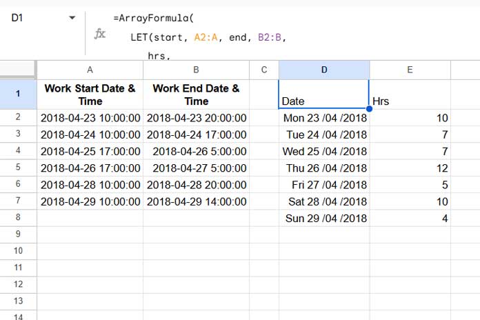
From the time sheet (refer screenshot # 1) I could successfully calculate the day wise working hours as above.

If an employee has started and ended his work on two different days, in day wise working hours calculation, his work time split between the days. Still didn’t get?

More About Calculating Day Wise Working Hours in Google Sheets

Below is the row # 5 and 6 data in my sample sheet. (refer screenshot # 1)

Row # 5:

04/25/18 17:00:00 | 04/26/18 5:00:00

Row # 6:

04/26/18 17:00:00 | 04/27/18 5:00:00

In this 26/04/2018 is Thursday. The employee worked total 12 hours on Thursday (refer screenshot # 2). How? In Row # 5 his work time on Thursday is 5 hours and in Row # 6 it’s 7 hours. Total 12 hours.

In Google Sheets you can calculate this type of Day Wise working hours with a single formula.

How to Calculate Day Wise Working Hours From Start and End Date and Time

If you have your employees start and end time entered in column A and B as per my sample data (refer screenshot # 1) you can use the below formula in Cell D2. There is no need for you to do anything extra.

I know it’s tough to read but useful if you follow my data format that mentioned above.

Formula #1:

={"Date","Total Hours";query(ArrayFormula(query({int(A3:A),query(IF(LEN(A3:A),(if(weekday(A3:A)<>WEEKDAY(B3:B),{(int(B3:B)-A3:A)*24,(B3:B-int(B3:B))*24},{((B3:B-A3:A)*24),MOD(ROW(B3:B),1)})),),"Select Col1");int(B3:B),query(IF(LEN(A3:A),(if(weekday(A3:A)<>WEEKDAY(B3:B),{(int(B3:B)-A3:A)*24,(B3:B-int(B3:B))*24},{((B3:B-A3:A)*24),MOD(ROW(B3:B),1)})),),"Select Col2")},"Select Col1,Col2 where Col2 is not null")),"Select Col1, Sum (Col2) group by Col1 label Sum(Col2)''")}

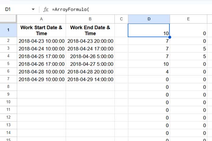
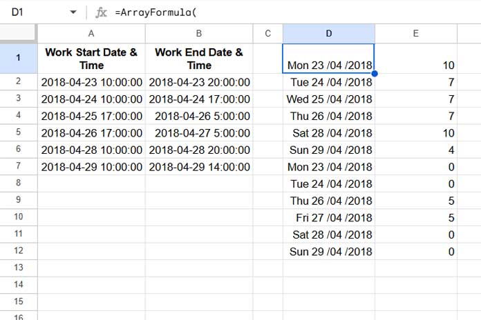
It’ll return the total working hours in day wise as per the above screenshot # 2. But do re type all double quotes in this formula to avoid parse error.

Screenshot # 3

Total Day Wise Work Hours in Array in Google Sheets

We have now the normal day wise working hours in column E. Now the next step is to calculate over time, weekend work time etc. from the above Column E values.

Before that let me explain you the above formula. If you are a beginner to Google Sheets or just want to use the template that I’m going to provide, you can skip this. For that reason, I’ve separated the explanation part with a separator line below. But I strongly suggest you to just read on to understand what the formula does.

You can access my example sheet Here. Open this file and then make a copy of it from the File menu. So that you will have an editable version of the file.


Formula Explanation: Day Wise Working Hours Calculation Formula in Google Sheets

Actually the above formula does a row wise summary. The formula finds the same days in different rows and total it. How?

For example I’m copying the above same data (screenshot # 1) in a new sheet tab and entering the following formula in Cell C3.

Note: If you want to learn all the Google Sheets functions mentioned in the nested formulas in this post, please refer my Google Sheets Functions Guide.

Formula #2:

=ArrayFormula(IF(LEN(A3:A),(if(weekday(A3:A)<>WEEKDAY(B3:B),{(int(B3:B)-A3:A)*24,(B3:B-int(B3:B))*24},{((B3:B-A3:A)*24),MOD(ROW(B3:B),1)})),))

See the output below.

Screenshot # 4:

Google Sheets: Split Shift Job Start and End Days

This formula calculates the total working hours from start time (time in) and end time (time out). It’s not limited to that. If the start time and end time dates are different, the formula simply split the working hours accordingly.

Related: Split Night Shift Job Hours into Two Columns

You can follow the above tutorial to know how this formula works. But one thing. There the formula generates total time duration instead of total hours.

That means the column C and Column D output will be time duration there. There is only minor changes in the last part of the formula.

You can place this formula # 2 and the formula detailed in the said tutorial side by side and compare to find the differences.

Now back to the tutorial. The above formula # 2 is the main part of the formula # 1. If you refer Screenshot # 4, you can see that the above formula # 2 returns two columns (Column C and D).

With a simple Google Sheets Query formula we can take the columns separate as below and there is a purpose behind that.

Formula # 3:

=query(ArrayFormula(IF(LEN(A3:A),(if(weekday(A3:A)<>WEEKDAY(B3:B),{(int(B3:B)-A3:A)*24,(B3:B-int(B3:B))*24},{((B3:B-A3:A)*24),MOD(ROW(B3:B),1)})),)),"Select Col1")

Formula # 4:

You can copy the same formula # 3 here. Then just change the Col1 to Col2. So I’m not copying the above formula here again.

Formula # 5:

The below generic formula is the basic of our formula # 1. In this, C2:C is formula # 3 and D2:D is formula # 4. I mean replace them with formula # 3 and #4 respectively.

ArrayFormula(query({int(A2:A),C2:C;int(B2:B),D2:D},"Select Col1,Col2 where Col2 is not null"))

What this generic version of the formula # 5 does?

Before explaining that please refer the screenshot # 4 above. Now I want that data in columns in the below order. The generic formula is used for this.

Column A and Column C in side by side and then make Column B and Column D in side by side and place them below Column A and C.

Further, I only want the dates in Column A and B. So to remove the time from date and time, I’ve used the INT function.

Here is the real formula of the generic version that does the column shuffling.

=ArrayFormula(query({int(A3:A),query(IF(LEN(A3:A),(if(weekday(A3:A)<>WEEKDAY(B3:B),{(int(B3:B)-A3:A)*24,(B3:B-int(B3:B))*24},{((B3:B-A3:A)*24),MOD(ROW(B3:B),1)})),),"Select Col1");int(B3:B),query(IF(LEN(A3:A),(if(weekday(A3:A)<>WEEKDAY(B3:B),{(int(B3:B)-A3:A)*24,(B3:B-int(B3:B))*24},{((B3:B-A3:A)*24),MOD(ROW(B3:B),1)})),),"Select Col2")},"Select Col1,Col2 where Col2 is not null"))

Output:

Screenshot 5:

date from date and time and hours

As you can see there are multiple occurrences of same dates in this output. So in the final formula (formula # 1) I’ve just summed the column 2 by grouping the dates in Column 1. This way you can calculate day wise working hours in Google Sheets.


We have calculated the day wise working hours. Now let’s see how to calculate normal working hours and over time working hours out from this.

Screenshot # 6:

In this please note that our formula # 1 is in Cell D2 and output in D2:E.

Exclude Weekends from Day Wise Working Hours

How to Exclude Weekends from Day Wise Working Hours.

Let me show you the formula in Cell G2 first.

Formula # 6:

={"Total Normal Hours";sum(ArrayFormula(IF(LEN(D3:D),if((weekday(D3:D)<>1)*(weekday(D3:D)<>7)>0,E3:E,),)))}

In this formula, the value 1 indicates Sunday and 7 indicates Saturday. These are weekend numbers. You can learn more about weekends in this Google Sheets date function guide.

This Google Sheets formula excludes the weekends from working hours and sum the total working hours. The total as per the above sample data is 41 hours.

Then what about weekends. I’ve considered the Weekend working hours as full over time.

How to Calculate Weekend Hours from Start and End Time

The working hours on weekends are considered as full over time in my calculation. To calculate the Weekend OT, the formula that I’ve used in the Cell H2 is as below.

Formula # 7:

={"Weekend Hours Total";sum(ArrayFormula(IF(LEN(D3:D),if((weekday(D3:D)=1)+(weekday(D3:D)=7)>0,E3:E,),)))}

And the total is 14 hours.

So as per the above two formulas the total working hours is;

Normal Day working + Weekends Working = 55 hours.

So now I am just deducting OT hours from normal day working hours (excluding weekends as weekends are already considered as full OT)

How to Calculate OT Hours from Start and End Time

I am talking about the formula in I2 which is as below.

Formula # 8:

={"Total OT Hours";sum(ArrayFormula(if(IF(LEN(D3:D),if((weekday(D3:D)<>1)*(weekday(D3:D)<>7)>0,E3:E,),)>8,E3:E-8,)))}

If an employee has worked more than 8 hours per day, I’ve considered the extra hours as OT hours. You can change both the occurrences of the number 8 in this formula to change the OT hours base.

I mean if an employee has worked 12 hours in a day, 8 hours is his normal working hours and 4 hours is his over time (OT). But I’ve excluded Weekends. I means in the above calculation I’ve excluded Saturday and Sunday.

Final Calculation:

In Cell H6:

Total Normal Hours – Total OT Hours (both excluding weekends) = Normal Pay Hour.

In Cell H7:

Weekend Hours + Total OT Hours = Total Over Time Pay Hour.

Screenshot # 7:

Normal + OT + Weekends

This is the method I’ve followed in my normal and OT hours calculations. You can change that based on the applicable rules in your country. The formula # 1 remains the same. You may only need to change the formulas used in Cell G2, H2, I2, G6 and G7.

Hope you could learn how to calculate day wise working hours, OT hours, night shift hours and weekend working hours using Google Sheets.

Prashanth KV
Prashanth KV
Your Trusted Google Sheets and Excel Guide Prashanth KV brings a wealth of experience in Google Sheets and Excel, cultivated through years of work with multinational corporations in Mumbai and Dubai. As a recognized Google Product Expert in Docs Editors, Prashanth shares his expertise through insightful blogging since 2012. Explore his blog for practical tips and guidance on maximizing your spreadsheet skills.

Lookup Values Under Categories in Excel and Google Sheets

We can use a combination of XLOOKUP and VLOOKUP in both Excel and Google...

Extract Items Under a Category from the Same Column in Excel

In Excel, you can use a combination of the XLOOKUP and DROP functions to...

How to Create a Searchable Table in Excel Using the FILTER Function

Finding specific records, or rows containing the required information, is straightforward in Excel using...

Time Sequences in Excel by Minute, Hour, or Second Increments

Creating time sequences, whether by hour, minute, or second increments in Excel, can be...

More like this

XMATCH Row by Row: Finding Values Across a Range in Google Sheets

Using the BYROW function with XMATCH in Google Sheets allows us to match values...

Limit Formula Expansion to a Specific Row in Google Sheets

In this tutorial, I’ll explain how to limit the expansion of an array formula...

3-D Referencing Structured Data Tables in Google Sheets

When you have several tables within a single sheet—not across multiple sheets in a...

9 COMMENTS

  1. Was there ever any follow-up to Mac’s issue? We need a similar thing. We have snowplow drivers that work consecutively 1-3 days, and we need to extract out the office hours of 7 am-3 pm so we can calculate overtime earned over multiple days.

    Any help would be greatly appreciated.

    Katie

  2. Oh man, thanks Prashanth for getting back to me so quickly, I hope there is a way around this. I’ve been wracking my brain (of limited spreadsheet knowledge) for days on this now – really hope you can solve this one 🙂 Thanks Again.

  3. Hi Prashanth, great spreadsheet.

    It is almost exactly what I need.

    However, my company must calculate different rates for night shift hours after a specific time in the evening too, not just after 8 hours of working.

    For example, weekdays between:
    – 8am to 5pm is £10p/hr,
    – 5pm to 11pm is £15p/hr and
    – 11pm to 8am is £20p/hr.

    How would we integrate this calculation into this exact same sheet including the weekend O.T rates you have shown above (FYI weekend rates are also charged at a higher rate than shift O.T hours for example:
    – 8am to 5pm is £15p/hr
    – 5pm to 11pm is £20p/hr
    – 11pm to 8am is £25p/hr

    • Hi, Mac,

      Sorry to say, this Sheet won’t work in that case because of the separate rate for working from 11 pm to 8 am.

      I may try to work on this problem later and link you here.

      Best,

  4. Thanks a lot for the information.

    In my company we have some break time throughout the day. Is it possible to exclude non working hours as well?

    • Hi, Ordan Gilboa,

      I guess the break time would be standard like 1 hour four lunch, 30 minutes for an evening break something like that for every day. Then we can do that.

      My formula returns total working hours in column range E3:E. So you can minus the break time directly from it using the below formula in cell F3.

      =ArrayFormula(if(len(D3:D),E3:E-1.5,))

      Format the column F to numbers from the menu Format > Number > Number.

      This formula subtracts 1.5 hours (1 hour 30 minutes) as a standard from the total working hours in each day. You can change this value as per your requirement.

      In cell G2, H2 and I2 change the cell reference E3:E to F3:F.

      I didn’t test this. But it must work.

LEAVE A REPLY

Please enter your comment!
Please enter your name here

This site uses Akismet to reduce spam. Learn how your comment data is processed.