Using a start and end time (timestamp), you can easily calculate daily working hours in Google Sheets, with the formula effectively handling cases where the start and end dates differ or include repeated dates.
The output will include a date column and an hours column. Using these, you can further analyze the data—for example, separating weekend hours, calculating overtime if an employee exceeds a specific number of hours in a day, etc. These additional tips are not included here but can be derived since the formula provides a detailed summary of working hours.
=ArrayFormula(
   LET(start, A2:A, end, B2:B,
      hrs,
      IF(
         INT(start)<>INT(end),
         HSTACK((INT(end)-start)*24,(end-INT(end))*24),
         N(IFNA(HSTACK(((end-start)*24),)))
      ),
      hrsDt,
      VSTACK(
         HSTACK(INT(start), CHOOSECOLS(hrs, 1)),
         HSTACK(INT(end), CHOOSECOLS(hrs, 2))
      ),
      QUERY(hrsDt, "SELECT Col1, SUM(Col2) WHERE Col2>0 GROUP BY Col1 LABEL Col1 'Date', SUM(Col2) 'Hrs'", 0)
   )
)
When using this formula, replace A3:A with your start datetime reference and B3:B with your end datetime reference.
To display the dates properly, select the first column of the result, then navigate to Format > Number > Date in Google Sheets.
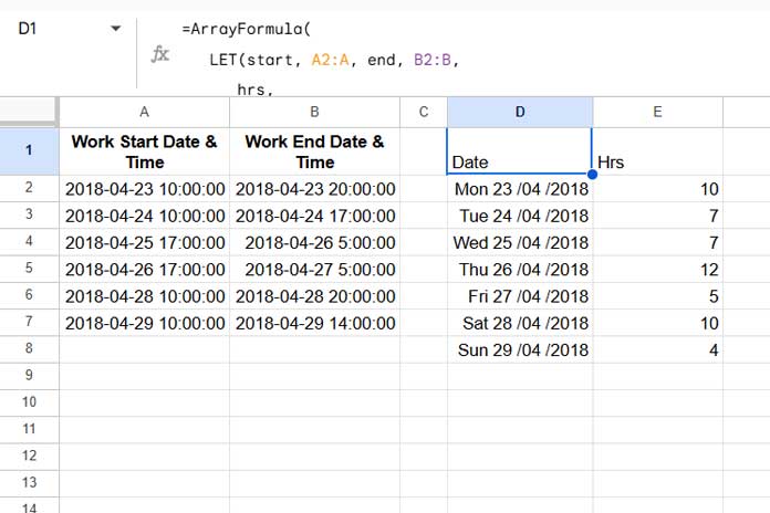
Example of Daily Working Hours Calculation
Sample Data in Columns A and B:
| Work Start Date & Time | Work End Date & Time |
| 2018-04-23 10:00:00 | 2018-04-23 20:00:00 |
| 2018-04-24 10:00:00 | 2018-04-24 17:00:00 |
| 2018-04-25 17:00:00 | 2018-04-26 5:00:00 |
| 2018-04-26 17:00:00 | 2018-04-27 5:00:00 |
| 2018-04-28 10:00:00 | 2018-04-28 20:00:00 |
| 2018-04-29 10:00:00 | 2018-04-29 14:00:00 |
- Column A contains the work start date and time (datetime format).
- Column B contains the work end date and time (datetime format).
It is essential to use the date and time format for accurate calculations, especially for jobs spanning multiple days (e.g., night shifts). For example, in the work start and end times provided above, some shifts begin on one day and end on the following day.
If you enter the formula in cell D1, it will output the total working hours grouped by dates:
How the Formula Calculates Daily Working Hours
The formula is broken into components using the LET function. Here’s how each component works:
Syntax of LET:
LET(name1, value_expression1, [name2, …], [value_expression2, …], formula_expression)Defined Names and Their Functions:
start: Refers to the start datetime range (A2:A).
end: Refers to the end datetime range (B2:B).
hrs: Calculates the working hours split across different dates:
Logic:
If INT(start) <> INT(end) (dates are different):
HSTACK( (INT(end)-start)*24, (end-INT(end) )*24) // calculates hours for the start and end dates separatelyElse:
N(IFNA(HSTACK(((end-start)*24),))) // calculates total hours for the same dateThe formula produces a two-column output, with Column 1 showing the hours worked on the start date and Column 2 showing the hours worked on the end date.
hrsDt:
VSTACK( HSTACK(INT(start), CHOOSECOLS(hrs, 1)), HSTACK(INT(end), CHOOSECOLS(hrs, 2)))Combines dates and hours into a two-column table using:
HSTACK(INT(start), CHOOSECOLS(hrs, 1)): Stacks the start date with the hours worked on that date.
HSTACK(INT(end), CHOOSECOLS(hrs, 2)): Stacks the end date with the hours worked on that date.
Finally, VSTACK merges these rows into one table.
- Formula Expression:
QUERY(hrsDt, "SELECT Col1, SUM(Col2) WHERE Col2>0 GROUP BY Col1 LABEL Col1 'Date', SUM(Col2) 'Hrs'", 0)The QUERY formula summarizes the working hours for each date by selecting rows where hours (Col2) > 0, grouping the data by the date column (Col1), and calculating the total daily working hours for each date.
Resources for Further Exploration
Here are additional tutorials to enhance your calculations in Google Sheets:
- How to Automate Overtime Calculation in Google Sheets
- Deducting Lunch Break Time From Total Hours In Google Sheets
- Combine Time In and Time Out into the Same Row in Google Sheets
- Elapsed Days and Time Between Two Dates in Google Sheets
- Group and Sum Time Duration Using Google Sheets Query
- Hourly Time Slot Booking Template in Google Sheets
- Excel Template for Hourly Time Slot Booking
- Free Automated Employee Timesheet Template for Google Sheets


Was there ever any follow-up to Mac’s issue? We need a similar thing. We have snowplow drivers that work consecutively 1-3 days, and we need to extract out the office hours of 7 am-3 pm so we can calculate overtime earned over multiple days.
Any help would be greatly appreciated.
Katie
Hi, Katie,
Can you please share real-life sample data in Sheet and your expected result? So that I can try ASAP.
Feel free to leave the URL below, which I won’t publish.
Hi, Katie,
I don’t have real-life sample data. For assistance, please prepare one and share that Sheet with me.
Oh man, thanks Prashanth for getting back to me so quickly, I hope there is a way around this. I’ve been wracking my brain (of limited spreadsheet knowledge) for days on this now – really hope you can solve this one 🙂 Thanks Again.
I will certainly try and update you.
Hi Prashanth, great spreadsheet.
It is almost exactly what I need.
However, my company must calculate different rates for night shift hours after a specific time in the evening too, not just after 8 hours of working.
For example, weekdays between:
– 8am to 5pm is £10p/hr,
– 5pm to 11pm is £15p/hr and
– 11pm to 8am is £20p/hr.
How would we integrate this calculation into this exact same sheet including the weekend O.T rates you have shown above (FYI weekend rates are also charged at a higher rate than shift O.T hours for example:
– 8am to 5pm is £15p/hr
– 5pm to 11pm is £20p/hr
– 11pm to 8am is £25p/hr
Hi, Mac,
Sorry to say, this Sheet won’t work in that case because of the separate rate for working from 11 pm to 8 am.
I may try to work on this problem later and link you here.
Best,
Thanks a lot for the information.
In my company we have some break time throughout the day. Is it possible to exclude non working hours as well?
Hi, Ordan Gilboa,
I guess the break time would be standard like 1 hour four lunch, 30 minutes for an evening break something like that for every day. Then we can do that.
My formula returns total working hours in column range E3:E. So you can minus the break time directly from it using the below formula in cell F3.
=ArrayFormula(if(len(D3:D),E3:E-1.5,))Format the column F to numbers from the menu Format > Number > Number.
This formula subtracts 1.5 hours (1 hour 30 minutes) as a standard from the total working hours in each day. You can change this value as per your requirement.
In cell G2, H2 and I2 change the cell reference E3:E to F3:F.
I didn’t test this. But it must work.