Some times you may require small tips to make your formulas work. Inserting a blank cell between two totals in a Query Total row in Google Sheets is one such small tip.

You can horizontally or vertically add a Query Total Row to a Query table output. My earlier two tutorials have in-depth details on this.

• Automatically Add Total to a Filtered Data in Google Sheets.
• How to Use QUERY Function Similar to Pivot Table in Google Sheets.

Here I am going to share a small tip that I have not addressed in those two tutorials. The tip is how to include a blank cell between two totals in a Query total row.

It may not be required at all times. But it will be useful at times (see the example screenshot below).

Actually the formula, not the tip, I’ve already shared with one of my readers as a reply to his comment (I’m not including that link).

This tutorial contains that formula, formula tip, and its explanation.

Example of Inserting a Blank Cell between Two Totals in a Query Total Row

Here is part of a sales data in A1:D.

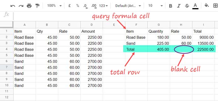
Since this tutorial contains step-by-step instructions (you will get the final formula in two main steps), you may please enter the same sample data in your sheet in the same range.

I’ve summarized the above part of the sales data (A1:D) by grouping column A (the items “Road Base” and “Sand”).

You can find the summary in the cell range F1:I (you will get the formula later).

In the summary, the aggregate columns are the columns B, C, and D. The columns B (Qty) and D (Amount) are summed and the column C (Rate) is averaged Query.

It’s obvious that we don’t want the total of the average column in the total row in the summary table. So in the Query total row, I want to skip the total of the average column C as you can see in the image above.

Here comes the importance of how to insert a blank cell between two totals in a Query total row in Google Sheets.

See the Query output in the range F1:I. You can see a blank cell between two totals in the Query total row in cell H4.

Let’s see how to insert a blank cell between two totals in the Query total row as above in Google Sheets.

There are two main steps. The first one is Query grouping and aggregation and the second one is Query total row.

Query Summary (Grouping and Aggregation)

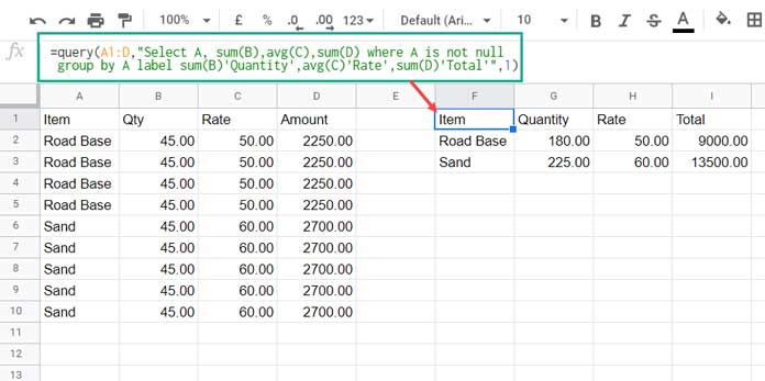
For the summary as per my explanation above, we can use the below QUERY formula which contains the Query aggregation functions Sum and Avg.

Query Summary Formula:

=query(
     A1:D,
     "Select A, sum(B),avg(C),sum(D) where A is not null group by A label sum(B)'Quantity',avg(C)'Rate',sum(D)'Total'",1
)

Formula Explanation (In a Nutshell)

We want to group column A. So included column A in the SELECT clause.

"Select A,

Then we should include the GROUP BY clause to group this column (all columns in the SELECT clause should find a place in the GROUP BY clause).

group by A

The columns B to be summed (SUM), C to be averaged (AVG), and again column D to be summed (SUM).

sum(B),avg(C),sum(D)

The QUERY ‘data’ is A1:D and we have data up to row#10 (A1:D10) only.

So I’ve included the below WHERE clause in the Query formula to avoid blank rows in the A1:D range. Othewise you will get a blank row in the Query summary table.

where A is not null

That means if the ‘data’ is A1:D10, you can skip the above clause in the formula.

Finally, the LABEL clause is to customize the labels of the Query summary output. You can skip it or use it.

label sum(B)'Quantity',avg(C)'Rate',sum(D)'Total'

You May Like: Understand the Label Clause in Google Sheets Query.

In the next step, you can learn the awesome tip to get a blank cell between two totals in a Query total row in Google Sheets.

Now we must use one more Query formula that to get the total row.

Get a Blank Cell (Column) between Two Totals in a Query Total Row

The total row should be in line with the above summary formula. So let’s copy the same formula and modify it. For the time being insert the Query (formula) in cell F4.

Remove the element A (column A) from the SELECT clause and also from the GROUP BY clause (remove the GROUP BY Clause). That’s the first thing that we should do.

=query(
     A1:D,
     "Select sum(B),avg(C),sum(D) where A is not null label sum(B)'Quantity',avg(C)'Rate',sum(D)'Total'",1
)

We will later combine this formula with our earlier Query formula (summary formula).

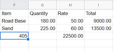
First of all, see the result and some sneak peek into what we are going to do in the comings steps (highlighted).

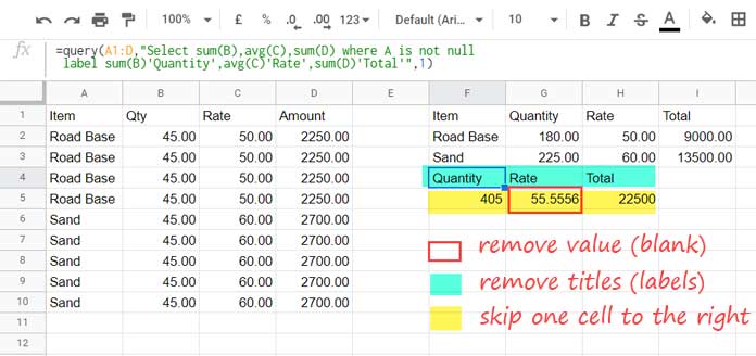
First I will start with the key tip.

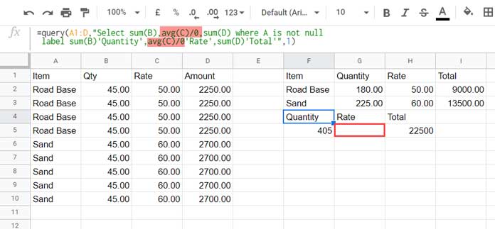
To get a blank cell, you can say column, between two totals in a Query total row use the ‘divide by zero methods’ with the corresponding aggregate function in use, here AVG.

In the above formula replace avg(C) with avg(C)/0. both in the aggregation part and label part.

This would result DIV/0! error in the corresponding total cell and that would be treated as a blank in Query.

=query(
     A1:D,
     "Select sum(B),avg(C)/0,sum(D) where A is not null label sum(B)'Quantity',avg(C)/0'Rate',sum(D)'Total'",1
)

Now let’s remove the labels. It’s quite simple.

You may simply remove the labels (but leave the open clause apostrophes) from the LABEL clause.

=query(
     A1:D,
     "Select sum(B),avg(C)/0,sum(D) where A is not null
 label sum(B)'',avg(C)/0'',sum(D)''",1
)

Finally to skip the total row one cell to the right, use the below technique.

Generic Formula:

={"TOTAL",above_query_formula}

Query Total Row Formula:

={
     "TOTAL",
     query(
        A1:D,
        "Select sum(B),avg(C)/0,sum(D) where A is not null
 label sum(B)'',avg(C)/0'',sum(D)''",1
     )
}

You will get the result as below.

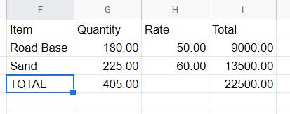
Let’s combine the above two formulas (summary formula and the Query total row formula).

Generic Formula:

{Query_Summary_Formula;Query_Total_Row_Formula}

Final Formula:

={
     query(
        A1:D,
        "Select A, sum(B),avg(C),sum(D) where A is not null group by A label sum(B)'Quantity',avg(C)'Rate',sum(D)'Total'",1
     );
     {
     "TOTAL",
     query(
        A1:D,
        "Select sum(B),avg(C)/0,sum(D) where A is not null label sum(B)'',avg(C)/0'',sum(D)''",1
     )
     }
}

This way you can insert a blank cell between two totals in a Query total row in Google Sheets.

Thanks for the stay. Enjoy!