The AVERAGEIFS function in Google Sheets is a statistical function with a logical flavor. It allows you to calculate the average of a range while applying multiple conditions. Unlike the simpler AVERAGEIF, which works with a single condition, AVERAGEIFS is designed for scenarios that require multiple criteria to filter the data.
If you only need to filter a table based on a single condition, the AVERAGEIF function is a simpler choice. However, if you need to apply multiple criteria, AVERAGEIFS is the function to use. That said, alternatives such as DAVERAGE or QUERY, along with combination formulas, can also achieve this purpose.
Syntax
AVERAGEIFS(average_range, criteria_range1, criterion1, [criteria_range2, criterion2, ...])- average_range: The range of cells containing the values you want to average.
- criteria_range1: The first range to which the first criterion applies.
- criterion1: The condition, pattern, or test to apply to criteria_range1.
- You can add additional criteria by specifying more criteria_range and criterion pairs.
Sample Data
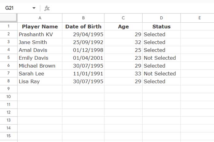
For this example, we’ll use the following sample data in columns A to D:

In this dataset, columns A to D represent player names, birthdates, ages, and their selection status.
Examples of Using the AVERAGEIFS Function
1. Single Criterion Example
The AVERAGEIFS function can be used with a single criterion, similar to AVERAGEIF. For example, to find the average age of players who are marked as “Selected”, use this formula:
=AVERAGEIFS(C2:C, D2:D, "Selected")C2:Ccontains the ages of players.D2:Dcontains the selection status (either “Selected” or “Not Selected”).
2. Multiple Criteria Example
To calculate the average age of players who are both “Selected” and older than 25, use this formula:
=AVERAGEIFS(C2:C, D2:D, "Selected", C2:C, ">25")This will return the average age of players who meet both criteria.
3. Using Comparison Operators in AVERAGEIFS
You can use various comparison operators (such as >, <, >=, <=, =) in your criteria. Here’s an example that calculates the average age of players whose names are not empty and their status is “Selected”:
=AVERAGEIFS(C2:C, A2:A, "<>", D2:D, "Selected")This formula ensures that it only averages the ages of players whose names are not blank and whose status is “Selected”.
4. Using Dates as Criteria in AVERAGEIFS
You can also use dates as criteria. The DATE function or the ISO 8601 format (yyyy-mm-dd) can be used. Here’s an example to calculate the average age of players born on or after January 1, 1995:
=AVERAGEIFS(C2:C, B2:B, ">="&DATE(1995, 1, 1))Alternatively, you can specify the date directly:
=AVERAGEIFS(C2:C, B2:B, ">=1995-01-01")Both formulas will return the average age of players born on or after January 1, 1995.
Can We Use OR Criteria in AVERAGEIFS?
In some situations, you may want to find the average based on multiple criteria in the same column, such as finding players who are either “Selected” or “Not Selected”. Unfortunately, AVERAGEIFS doesn’t directly support the OR condition. For example, the following formula would return a #DIV/0! error:
AVERAGEIFS(C2:C, D2:D, "Selected", D2:D, "Not Selected")To achieve this behavior, use ARRAYFORMULA combined with the following formula:
=ARRAYFORMULA(AVERAGEIFS(C2:C, (D2:D="Selected")+(D2:D="Not Selected"), 1))Here’s what happens:
(D2:D="Selected") + (D2:D="Not Selected")creates an array ofTRUEandFALSEvalues. When summed,TRUEbecomes1andFALSEbecomes0.- The ARRAYFORMULA function processes this array, allowing the AVERAGEIFS function to handle multiple criteria as OR conditions.
Additional Tips:
You can replace AVERAGEIFS with QUERY or a combination of FILTER and AVERAGE for more complex filtering scenarios. In a structured dataset, you can also use DAVERAGE. Understanding these functions will expand your ability to filter and average data dynamically.
You can explore more about these functions in my Google Sheets Function Guide.
Resources
- AVERAGEIFS ArrayFormula Using MMULT in Google Sheets (Date Range)
- Average of Top N Percent of the Values in Google Sheets – With or Without Conditions
- Find the Average of the Last N Values in Google Sheets
- Average by Month in Google Sheets (Formula Options)
- Average of Smallest N Values in Google Sheets (Zero and Non-Zero)
- How to Calculate Average by Quarter in Google Sheets


