")
")


")


")

")
")
 in Excel & Google Sheets")


The main purpose of using Named Ranges is to create clean, readable formulas. But they won’t help much with ever-expanding datasets—unless you know how to auto-expand Named Ranges in Google Sheets.
Fortunately, there’s a simple workaround to make Named Ranges dynamic. In this guide, I’ll walk you through step-by-step instructions so you can master this technique with ease.
Before we dive in, let’s cover the basics.
Basic Example of Creating a Named Range in Google Sheets
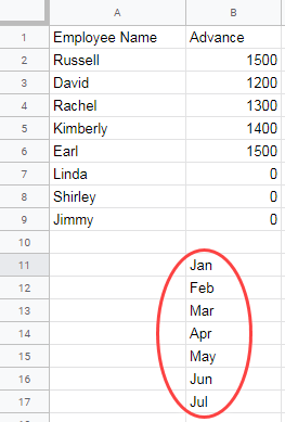
In the screenshot below, column B contains the advance payments made to a few employees. The data range is B2:B9.
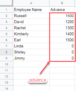
If you name this range "advance", your formulas become much simpler. For example:
=SUM(advance)instead of:
=SUM(B2:B9)To name the range B2:B9, just follow these steps:
- Select B2:B9.
- Go to Data > Named ranges.
- Enter the name advance.
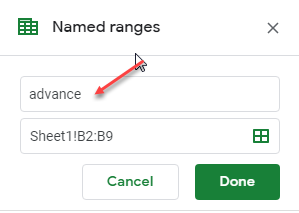
That’s it—your range is now easier to use.
But here’s the catch: if your data grows, a static Named Range won’t update automatically. That’s where an auto-expanding Named Range becomes essential.
Why You Need Auto-Expanding Named Ranges in Google Sheets
Reason 1:
Continuing with the above example—if you add a new entry in row 10, the Named Range formula won’t capture it. You’ll need to manually edit the range from Data > Named ranges, which is tedious and prone to mistakes.
Reason 2:
You might think of future-proofing by extending the range to B2:B1000. While it works, it also includes hundreds of empty cells, which can cause performance issues and inefficient calculations.
This highlights the need for dynamic Named Ranges in Google Sheets that grow automatically.
Creating an auto-expanding Named Range depends on whether your data is one-dimensional (a column or a row) or two-dimensional (a table). Let’s look at both cases.
How to Create Auto-Expanding Named Ranges for a Column
Here’s how you can set it up step by step.
Step 1: Use This Formula
=LET(
   col, B2:B,
   sheet_name, "Sheet1",
   l_test, ARRAYFORMULA(ISBLANK(col)),
   start, CELL("address", XLOOKUP(FALSE, l_test, col,, 0, 1)),
   end, CELL("address", XLOOKUP(FALSE, l_test, col,, 0, -1)),
   sheet_name & "!" & start & ":" & end
)
Formula Explanation
ARRAYFORMULA(ISBLANK(col)): Returns TRUE for blank cells and FALSE for filled cells.XLOOKUP(FALSE, l_test, col,, 0, 1): Finds the first non-blank cell (top to bottom).XLOOKUP(FALSE, l_test, col,, 0, -1): Finds the last non-blank cell (bottom to top).CELL("address", …): Gets the addresses of those cells.- Finally, the formula joins the sheet name and addresses into a usable range.
👉 You’ll need to adjust:
- Sheet1 → your sheet’s name.
- B2:B → your actual column range.
Note: By default, this formula creates a range from the first non-blank cell to the last non-blank cell in B2:B. If you want the range to always begin at B2 (even if B2 is blank), replace CELL("address", XLOOKUP(FALSE, l_test, col,, 0, 1)) with "B2".
Step 2: Create a Named Range Using a Helper Cell
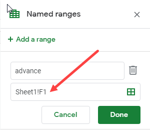
- Enter the formula above in a helper cell (say, F1).
- Go to Data > Named ranges and create a Named Range called
advance. - Point it to F1 instead of B2:B9.
Now, instead of:
=SUM(advance)use:
=SUM(INDIRECT(advance))Your Named Range will now auto-update whenever new rows are added.
👉 Note: You can skip Named Ranges and use INDIRECT(F1), but Named Ranges are easier to read and work across the workbook.
How to Create Auto-Expanding Named Ranges for a Row
The same formula works for horizontal ranges too.
For example, to make B2:Z2 dynamic, just replace B2:B with B2:Z2 in the formula.
If you want the range to always start from B2, replace the CELL("address", XLOOKUP(FALSE, l_test, col,, 0, 1)) part with "B2".
How to Create Auto-Expanding Named Ranges for a 2D Array
Suppose you have sales data in A1:E6 of Sheet1, where column A lists salespersons and the other columns store sales quantities:

You want to create a dynamic Named Range called sales_data that grows both vertically and horizontally as new data is added.
Use this formula in another sheet (to avoid circular references) and then use that helper cell to create the dynamic 2D Named Range.
=ArrayFormula(LET(
  range, Sheet1!A1:Z,
  start, ADDRESS(MIN(ROW(range)), MIN(COLUMN(range)), 4),
  colL, REGEXEXTRACT(ADDRESS(1,
    LET(
      range_, range,
      bt, NOT(ISBLANK(range_)),
      errv, IF(bt, bt, NA()),
      rseq, SEQUENCE(COLUMNS(errv), 1, -1, -1),
      swap, CHOOSECOLS(errv, rseq),
      row_, SORTN(swap),
      id, XMATCH(TRUE, row_),
      COLUMNS(range_)-id+COLUMN(INDIRECT(start))
    )
  ), "[A-Z]+"),
  rowN,
    LET(
      range_, TRANSPOSE(range),
      bt, NOT(ISBLANK(range_)),
      errv, IF(bt, bt, NA()),
      rseq, SEQUENCE(COLUMNS(errv), 1, -1, -1),
      swap, CHOOSECOLS(errv, rseq),
      row_, SORTN(swap),
      id, XMATCH(TRUE, row_),
      COLUMNS(range_)-id+ROW(INDIRECT(start))
    ),
  JOIN(, "Sheet1!", start, ":", colL, rowN)
))
Here’s what’s happening:
- The formula checks for the last non-blank row and column.
- It finds the bottom-right cell and returns a dynamic range from the top-left cell to that cell (the actual used range).
- Your Named Range grows automatically when new data is added in rows or columns.
👉 Replace Sheet1!A1:Z with the maximum expected growth area of your data.
For details, see my full tutorial: How to Find the Bottom-Right Corner of Your Data in Google Sheets.
Limitations of Auto-Expanding Named Ranges in Google Sheets
No guide is complete without discussing caveats:
- Columns: If there are values below your intended dataset, they will be included in the Named Range.
- Rows: The same applies if there are values beyond your intended row range.
- 2D Arrays: Must be used in a different sheet to prevent circular references.
Frequently Asked Questions (FAQ)
Q1. Can Named Ranges automatically expand in Google Sheets?
Not directly. By default, Named Ranges in Google Sheets are static. However, you can use formulas with LET, XLOOKUP, and CELL to create auto-expanding Named Ranges that adjust when new rows or columns are added.
Q2. How do I make a Named Range dynamic in Google Sheets?
You can make a Named Range dynamic by first creating a helper formula (for example, one that calculates the first and last non-blank cells in a column) and then assigning that formula result as the Named Range. When you add new data, the Named Range automatically includes it.
Q3. What are the limitations of auto-expanding Named Ranges?
The main limitation is that unwanted values outside your dataset (extra rows or columns) may get included in the Named Range. Also, for 2D ranges, the formula must be placed outside the dataset or on another sheet to avoid circular reference errors.
Additional Resources
- How to View Named Ranges in Google Sheets [Quick Tips]
- How to Use Named Ranges in QUERY in Google Sheets
- Mastering SUMIF with Named Ranges in Google Sheets
- Using Named Ranges in VLOOKUP in Google Sheets
- IMPORTRANGE Named Ranges in Google Sheets – A Complete Guide
- Dynamic Column ID in QUERY IMPORTRANGE Using Named Range
- Highlighting Named Ranges in Google Sheets
- How to Use Named Ranges in Conditional Formatting in Google Sheets
Thank you very much for your formula! The only nuance, of course, is that I have to wrap all the names of ranges in INDIRECT, which slightly worsens readability in complex formulas. But here I understand that I have to wait for Google’s solution, because there is no other way to solve it.
Hi Prashanth, this formula is very useful to create a dynamic named range in google sheets.
But there is a problem that we won’t be able to use this named range in a data validation drop-down list.
It always shows to input a valid range.
Hi, jeetendra,
That’s correct in the case of data validation as it won’t accept formulas.
This is just the function that I need! Thank you! If I have a fixed number of columns, but many, not just 1, and expanding rows, how can I include the whole range of columns with ever-expanding rows?
Hi, Hope,
Here is the helper cell (cell F1) formula in my tutorial.
="Sheet1!B2:"&"B"&match(2,ArrayFormula(1/(B1:B<>"")),1)This auto-expanding named range is for the cell range B2:B.
For cell range B2:D (multiple columns), just change the formula in cell F1 as below.
="Sheet1!B2:"&"D"&match(2,ArrayFormula(1/(B1:B<>"")),1)But it has one issue. It will only check for the last value in column B. To consider all the columns, you may need to modify the formula as below.
="Sheet1!B2:"&"D"&match(2,ArrayFormula(1/(B1:B&C1:C&D1:D<>"")),1)Thanks for your easy to understand guide! Very well written.
I’m stuck now as I wish to use the named range for more complex functions that sum.
Can it be used for countifs?
e.g.
=countifs(indirect(Advancerange1,criteraA,Advancerange2,criteriaB))I get
“Error
Wrong number of arguments to COUNTIFS. Expected at least 2 arguments, but received 1 arguments.”
I wish there was a way to use your trick without indirect..
It seems I cannot use multiple criteria and also I will have to update all my functions adding indirect.
Do you have any advice?
Hi, mava,
You can definitely use dynamic named ranges in functions like Sumif, Sumifs, Countif, Countifs, Query, etc. Here is one example using Countifs.
=countifs(indirect(Advancerange1),"=5",indirect(Advancerange2),"=5")Please note one thing! In the dynamic ranges, the Match formula must be based on the same column.
For example, in the above formula the “Advancerange1” range is B2:B and “Advancerange2” is C2:C.
My dynamic range of helper cells are H1 and G1 respectively. Here are the corresponding formulas in cell H1 and G1.
H1:
="Sheet1!B2:"&"B"&match_formula_hereG1:
="Sheet1!C2:"&"C"&match_formula_hereIn both of these formulas, use the same Match formula mentioned in the tutorial, i.e based on column B.
In short, in dynamic range only use the same column in the Match formula part.
Hi! Thanks for your website, I find it useful!
Wanted to add to your formula, that if my range, for example, starts not from the first row (4 in my case), in that case, you need to add the offset number of rows (+3 in my case) to the Match formula result, or in other cases, it will calculate the last row wrongly, found this out by logically analyzing the formula
Example:
="Sheet1!B4:"&"B"&match(2,ArrayFormula(1/(B4:B"")),1)+3Could you apply this method to create a dynamic named range if the range existed across columns rather than rows? Any feedback is greatly appreciated. Really enjoyed this demo, thanks!
First I thought it’s easy to code. But there is a real challenge in writing the formula. Here it is!
DYNAMIC NAMED RANGE ACROSS COLUMNS:
I am considering the dynamic named range in A3:G3 for the explanation below. The concerned formula is in cell A9.
1. In the formula in cell A9, you can see the text
Sheet1!A3. In that changeSheet1with your original Sheet’s name.2. In the same text replace A3 with the starting column. For example, if you want a dynamic range from B3, change A3 with B3.
To understand other changes when the row changes, please compare the two auto-expanding (dynamic) named range formulas.
Why not use “F1” instead of “advance”? I think its the same.